Welch’s Two Sample T-tests in R
- 1 Test Statistic for Welch’s Two Sample T-test in R
- 2 Simple Welch’s Two Sample T-test in R
- 3 Welch’s Two Sample T-test Critical Value in R
- 4 Two-tailed Welch’s Two Sample T-test in R
- 5 One-tailed Welch’s Two Sample T-test in R
- 6 Welch’s Two Sample T-test: Test Statistics, P-value & Degree of Freedom in R
- 7 Welch’s Two Sample T-test: Estimates, Standard Error & Confidence Interval in R
Here, we discuss Welch’s two sample t-test in R with interpretations, including, test statistics, p-values, critical values, confidence intervals, and standard errors.
The Welch’s two sample t-test in R can be performed with the
t.test() function from the base "stats" package.
The Welch’s two sample t-test is also the independent (unpaired) two sample t-test with unequal variance assumption. It can be used to test whether the difference between the means of the two populations where two independent random samples come from is equal to a certain value (which is stated in the null hypothesis) or not.
In the Welch’s two sample t-test, the test statistic follows a Student’s t-distribution when the null hypothesis is true.
| Question | Are the means equal, or difference equal to \(\mu_0\)? | Is mean x greater than mean y, or difference greater than \(\mu_0\)? | Is mean x less than mean y, or difference less than \(\mu_0\)? |
| Form of Test | Two-tailed | Right-tailed test | Left-tailed test |
| Null Hypothesis, \(H_0\) | \(\mu_x = \mu_y;\) \(\quad\) \(\mu_x - \mu_y = \mu_0\) | \(\mu_x = \mu_y;\) \(\quad\) \(\mu_x-\mu_y = \mu_0\) | \(\mu_x = \mu_y;\) \(\quad\) \(\mu_x-\mu_y = \mu_0\) |
| Alternate Hypothesis, \(H_1\) | \(\mu_x \neq \mu_y;\) \(\quad\) \(\mu_x-\mu_y \neq \mu_0\) | \(\mu_x > \mu_y;\) \(\quad\) \(\mu_x-\mu_y > \mu_0\) | \(\mu_x < \mu_y;\) \(\quad\) \(\mu_x-\mu_y < \mu_0\) |
Sample Steps to Run a Welch Two Sample T-test:
# Create the data samples for the Welch two sample t-test

data_x = c(5.1, 2.0, 4.1, 6.2, 7.1, 8.3)
data_y = c(1.5, 6.4, 3.3, 5.8,
           4.8, 7.2, 5.6, 4.5)

# Run the Welch two sample t-test with specifications

t.test(data_x, data_y,
       alternative = "two.sided",
       mu = 0, conf.level = 0.95)
    Welch Two Sample t-test

data:  data_x and data_y
t = 0.51703, df = 9.48, p-value = 0.617
alternative hypothesis: true difference in means is not equal to 0
95 percent confidence interval:
 -1.935420  3.093754
sample estimates:
mean of x mean of y
5.466667 4.887500 | Argument | Usage |
| x, y | The two sample data values |
| x ~ y | x contains the two sample data values, y specifies the group they belong |
| alternative | Set alternate hypothesis as "greater", "less", or the default "two.sided" |
| mu | The difference between the population mean values in null hypothesis |
| conf.level | Level of confidence for the test and confidence interval (default = 0.95) |
Creating a Welch Two Sample T-test Object:
# Create data
data_x = rnorm(90); data_y = rnorm(150)

# Create object
test_object = t.test(data_x, data_y,
                     alternative = "two.sided",
                     mu = 0, conf.level = 0.95)

# Extract a component
test_object$statistic
t
0.7463572 | Test Component | Usage |
| test_object$statistic | t-statistic value |
| test_object$p.value | P-value |
| test_object$parameter | Degrees of freedom |
| test_object$estimate | Point estimates or sample means |
| test_object$stderr | Standard error value |
| test_object$conf.int | Confidence interval |
1 Test Statistic for Welch’s Two Sample T-test in R
The Welch’s two sample t-test given its independent samples and unequal variance assumption has test statistics, \(t\), of the form:
\[t = \frac{(\bar x - \bar y) - \mu_0}{\sqrt{\frac{s_x^2}{n_x} + \frac{s_y^2}{n_y}}}.\] For independent random samples that come from normal distributions or for large sample sizes (for example, \(n_x > 30\) and \(n_y > 30\)), \(t\) is said to follow the Student’s t-distribution when the null hypothesis is true, with the degrees of freedom as \(\frac{\left(\frac{s_x^2}{n_x} + \frac{s_y^2}{n_y}\right)^2}{\frac{\left(s_x^2/n_x\right)^2}{n_x-1} + \frac{\left(s_y^2/n_y\right)^2}{n_y-1}}\).
\(\bar x\) and \(\bar y\) are the sample means,
\(\mu_0\) is the difference between the population mean values to be tested and set in the null hypothesis,
\(s_x\) and \(s_y\) are the sample standard deviations,
\(s_x^2\) and \(s_y^2\) are the sample variances, and
\(n_x\) and \(n_y\) are the sample sizes.
See also one sample t-tests and two sample t-tests (independent & equal variance and dependent or paired samples).
2 Simple Welch’s Two Sample T-test in R
Enter the data by hand.
data_x = c(19.1, 21.0, 17.5, 22.1, 17.0,
          19.2, 19.1, 22.7, 21.2, 23.3,
          18.2, 19.1, 22.2, 20.0, 19.3)
data_y = c(17.9, 18.8, 19.1, 21.4, 18.1,
          22.6, 16.0, 19.9, 15.8, 22.3)
For data_x as the \(x\) group and data_y as the \(y\) group.
For the following null hypothesis \(H_0\), and alternative hypothesis \(H_1\), with the level of significance \(\alpha=0.05\).
\(H_0:\) the difference between the population means is equal to 0 (\(\mu_x - \mu_y = 0\)).
\(H_1:\) the difference between the population means is not equal to 0 (\(\mu_x - \mu_y \neq 0\), hence the default two-sided).
Because the level of significance is \(\alpha=0.05\), the level of confidence is \(1 - \alpha = 0.95\).
The t.test() function has the default
alternative as "two.sided", the default difference
between the means as 0, and the default level of
confidence as 0.95, hence, you do not need to specify the
"alternative", "mu", and "conf.level" arguments in this
case.
Or:
    Welch Two Sample t-test

data:  data_x and data_y
t = 0.96948, df = 16.488, p-value = 0.3463
alternative hypothesis: true difference in means is not equal to 0
95 percent confidence interval:
 -1.035682  2.789015
sample estimates:
mean of x mean of y
 20.06667  19.19000
The first sample mean, \(\bar x\), is 20.06667, and the second sample mean, \(\bar y\), is 19.19000,
test statistic, \(t\), is 0.96948,
the degrees of freedom, \(\frac{\left(\frac{s_x^2}{n_x} + \frac{s_y^2}{n_y}\right)^2}{\frac{\left(s_x^2/n_x\right)^2}{n_x-1} + \frac{\left(s_y^2/n_y\right)^2}{n_y-1}}\), is 16.488,
the p-value, \(p\), is 0.3463,
the 95% confidence interval is [-1.035682, 2.7890151].
Interpretation:
P-value: With the p-value (\(p = 0.3463\)) being greater than the level of significance 0.05, we fail to reject the null hypothesis that the difference between the population means is equal to 0.
\(t\)-statistic: With test statistics value (\(t = 0.96948\)) being between the two critical values, \(-t_{df, \alpha/2}=\text{qt(0.025, 16.488)}=-2.1148174\) and \(t_{df, \alpha/2}=\text{qt(0.975, 16.488)}=2.1148174\) (or not in the shaded region), we fail to reject the null hypothesis that the difference between the population means is equal to 0.
Confidence Interval: With the null hypothesis difference between the population means value (\(\mu_x - \mu_y = 0\)) being inside the confidence interval, \([-1.035682, 2.7890151]\), we fail to reject the null hypothesis that the difference between the population means is equal to 0.
x = seq(-4, 4, 1/1000); y = dt(x, df=16.488)
plot(x, y, type = "l",
     xlim = c(-4, 4), ylim = c(-0.03, max(y)),
     main = "Welch's Two Sample Student's T-test
Shaded Region for Simple T-test",
     xlab = "x", ylab = "Density",
     lwd = 2, col = "blue")
abline(h=0)
# Add shaded region and legend
point1 = qt(0.025, 16.488); point2 = qt(0.975, 16.488)
polygon(x = c(-4, x[x <= point1], point1),
        y = c(0, y[x <= point1], 0),
        col = "blue")
polygon(x = c(x[x >= point2], 4, point2),
        y = c(y[x >= point2], 0, 0),
        col = "blue")
legend("topright", c("Area = 0.05"),
       fill = c("blue"), inset = 0.01)
# Add critical value and t-value
arrows(0, 0.1, 0.96948, 0)
text(0, 0.12, "t = 0.96948")
text(-2.114817, -0.02, expression(-t[df][','][alpha/2]==-2.114817))
text(2.114817, -0.02, expression(t[df][','][alpha/2]==2.114817))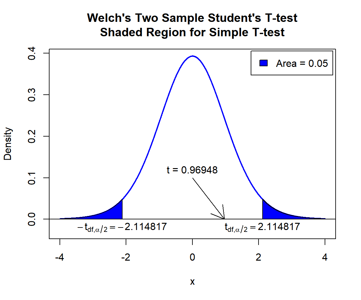
Welch’s Two Sample Student’s T-test Shaded Region for Simple T-test in R
See line charts, shading areas under a curve, lines & arrows on plots, mathematical expressions on plots, and legends on plots for more details on making the plot above.
3 Welch’s Two Sample T-test Critical Value in R
To get the critical value for a Welch’s two sample t-test in R, you
can use the qt() function for Student’s t-distribution to
derive the quantile associated with the given level of significance
value \(\alpha\).
For two-tailed test with level of significance \(\alpha\). The critical values are: qt(\(\alpha/2\), df) and qt(\(1-\alpha/2\), df).
For one-tailed test with level of significance \(\alpha\). The critical value is: for left-tailed, qt(\(\alpha\), df); and for right-tailed, qt(\(1-\alpha\), df).
Example:
For \(\alpha = 0.1\), and \(\text{df = 42.5}\).
Two-tailed:
[1] -1.681506[1] 1.681506One-tailed:
[1] -1.301791[1] 1.3017914 Two-tailed Welch’s Two Sample T-test in R
Using the ToothGrowth data from the "datasets" package with 10 sample rows from 60 rows below:
    len supp dose
1   4.2   VC  0.5
5   6.4   VC  0.5
23 33.9   VC  2.0
25 26.4   VC  2.0
30 29.5   VC  2.0
36 10.0   OJ  0.5
44 26.4   OJ  1.0
49 14.5   OJ  1.0
52 26.4   OJ  2.0
60 23.0   OJ  2.0
For OJ as the \(x\) group versus VC as the \(y\) group.
For the following null hypothesis \(H_0\), and alternative hypothesis \(H_1\), with the level of significance \(\alpha=0.1\).
\(H_0:\) population mean of group \(x\) minus population mean of group \(y\) is equal to 7.5 (\(\mu_x - \mu_y = 7.5\)).
\(H_1:\) population mean of group \(x\) minus population mean of group \(y\) is not equal to 7.5 (\(\mu_x - \mu_y \neq 7.5\), hence the default two-sided).
Because the level of significance is \(\alpha=0.1\), the level of confidence is \(1 - \alpha = 0.9\).
# This example uses t.test(x ~ y). For t.test(x, y), see other examples above or below.
t.test(len ~ supp, data = ToothGrowth,
       alternative = "two.sided",
       mu = 7.5, conf.level = 0.9)
    Welch Two Sample t-test

data:  len by supp
t = -1.967, df = 55.309, p-value = 0.0542
alternative hypothesis: true difference in means between group OJ and group VC is not equal to 7.5
90 percent confidence interval:
 0.4682687 6.9317313
sample estimates:
mean in group OJ mean in group VC
        20.66333         16.96333
Interpretation:
P-value: With the p-value (\(p = 0.0542\)) being lower than the level of significance 0.1, we reject the null hypothesis that the difference between the population means is equal to 7.5.
\(t\)-statistic: With test statistics value (\(t = -1.967\)) being inside the critical region (shaded area), that is, \(t = -1.967\) less than \(-t_{df, \alpha/2}=\text{qt(0.05, 55.309)}=-1.6728739\), we reject the null hypothesis that the difference between the population means is equal to 7.5.
Confidence Interval: With the null hypothesis difference between the population means value (\(\mu_x - \mu_y = 7.5\)) being outside the confidence interval, \([0.4682687, 6.9317313]\), we reject the null hypothesis that the difference between the population means is equal to 7.5.
x = seq(-4, 4, 1/1000); y = dt(x, df=55.309)
plot(x, y, type = "l",
     xlim = c(-4, 4), ylim = c(-0.03, max(y)),
     main = "Welch's Two Sample Student's T-test
Shaded Region for Two-tailed Test",
     xlab = "x", ylab = "Density",
     lwd = 2, col = "blue")
abline(h=0)
# Add shaded region and legend
point1 = qt(0.05, 55.309); point2 = qt(0.95, 55.309)
polygon(x = c(-4, x[x <= point1], point1),
        y = c(0, y[x <= point1], 0),
        col = "blue")
polygon(x = c(x[x >= point2], 4, point2),
        y = c(y[x >= point2], 0, 0),
        col = "blue")
legend("topright", c("Area = 0.1"),
       fill = c("blue"), inset = 0.01)
# Add critical value and t-value
arrows(-1.967, 0.2, -1.967, 0)
text(-1.967, 0.22, expression(t==-1.967))
text(-1.672874, -0.02, expression(-t[df][','][alpha/2]==-1.672874))
text(1.672874, -0.02, expression(t[df][','][alpha/2]==1.672874))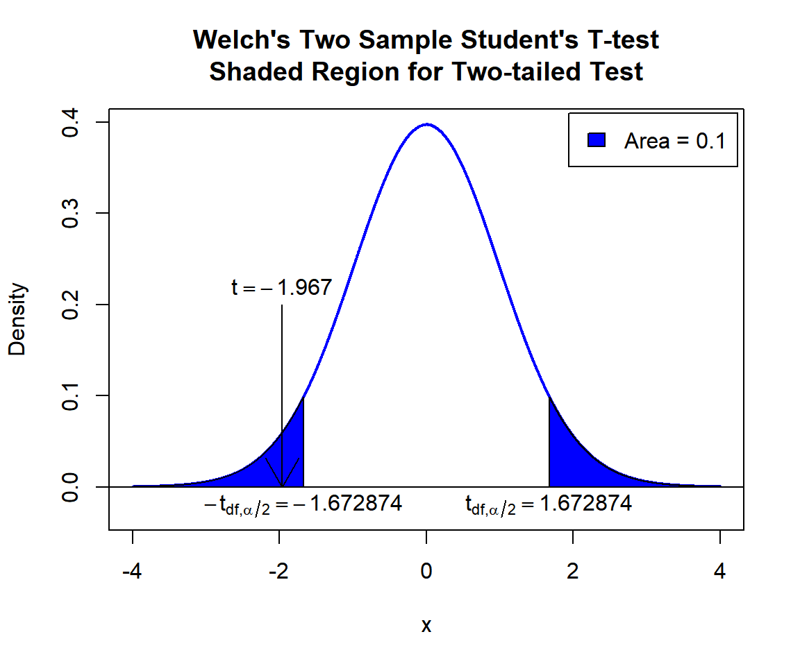
Welch’s Two Sample Student’s T-test Shaded Region for Two-tailed Test in R
5 One-tailed Welch’s Two Sample T-test in R
Right Tailed Test
Using the attitude data from the "datasets" package with 10 sample rows from 30 rows below:
   rating complaints privileges learning raises critical advance
1      43         51         30       39     61       92      45
4      61         63         45       47     54       84      35
11     64         53         53       58     58       67      34
12     67         60         47       39     59       74      41
15     77         77         54       72     79       77      46
16     81         90         50       72     60       54      36
19     65         70         46       57     75       85      46
20     50         58         68       54     64       78      52
23     53         66         52       50     63       80      37
30     82         82         39       59     64       78      39
For "complaints" as the \(x\) group versus "privileges" as the \(y\) group.
For the following null hypothesis \(H_0\), and alternative hypothesis \(H_1\), with the level of significance \(\alpha=0.15\).
\(H_0:\) population mean of group \(x\) minus population mean of group \(y\) is equal to 8 (\(\mu_x - \mu_y = 8\)).
\(H_1:\) population mean of group \(x\) minus population mean of group \(y\) is greater than 8 (\(\mu_x - \mu_y > 8\), hence one-sided).
Because the level of significance is \(\alpha=0.15\), the level of confidence is \(1 - \alpha = 0.85\).
t.test(attitude$complaints, attitude$privileges,
       alternative = "greater",
       mu = 8, conf.level = 0.85)
    Welch Two Sample t-test

data:  attitude$complaints and attitude$privileges
t = 1.6558, df = 57.59, p-value = 0.0516
alternative hypothesis: true difference in means is greater than 8
85 percent confidence interval:
 10.01384      Inf
sample estimates:
mean of x mean of y
 66.60000  53.13333
Interpretation:
P-value: With the p-value (\(p = 0.0516\)) being lower than the level of significance 0.15, we reject the null hypothesis that the difference between the population means is equal to 8.
\(t\)-statistic: With test statistics value (\(t = 1.6558\)) being inside the critical region (shaded area), that is, \(t = 1.6558\) greater than \(t_{df, \alpha}=\text{qt(0.85, 57.59)}=1.0458505\), we reject the null hypothesis that the difference between the population means is equal to 8.
Confidence Interval: With the null hypothesis difference between the population means value (\(\mu_x - \mu_y = 8\)) being outside the confidence interval, \([10.01384, \infty)\), we reject the null hypothesis that the difference between the population means is equal to 8.
x = seq(-4, 4, 1/1000); y = dt(x, df=57.59)
plot(x, y, type = "l",
     xlim = c(-4, 4), ylim = c(-0.03, max(y)),
     main = "Welch's Two Sample Student's T-test
Shaded Region for Right-tailed Test",
     xlab = "x", ylab = "Density",
     lwd = 2, col = "blue")
abline(h=0)
# Add shaded region and legend
point = qt(0.85, 57.59)
polygon(x = c(x[x >= point], 4, point),
        y = c(y[x >= point], 0, 0),
        col = "blue")
legend("topright", c("Area = 0.15"),
       fill = c("blue"), inset = 0.01)
# Add critical value and t-value
arrows(1.6558, 0.25, 1.6558, 0)
text(1.6558, 0.27, expression(t==1.6558))
text(1.04585, -0.02, expression(t[df][','][alpha]==1.04585))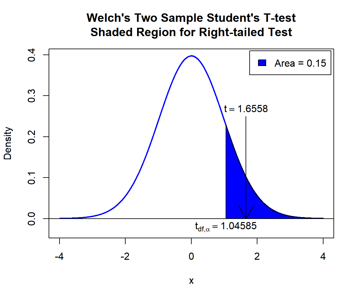
Welch’s Two Sample Student’s T-test Shaded Region for Right-tailed Test in R
Left Tailed Test
For "rating" as the \(x\) group versus "complaints" as the \(y\) group.
For the following null hypothesis \(H_0\), and alternative hypothesis \(H_1\), with the level of significance \(\alpha=0.05\).
\(H_0:\) population mean of group \(x\) and population mean of group \(y\) are equal (\(\mu_x - \mu_y = 0\)).
\(H_1:\) population mean of group \(x\) is less than population mean of group \(y\) (\(\mu_x - \mu_y < 0\), hence one-sided).
Because the level of significance is \(\alpha=0.05\), the level of confidence is \(1 - \alpha = 0.95\).
    Welch Two Sample t-test

data:  attitude$rating and attitude$complaints
t = -0.5971, df = 57.54, p-value = 0.2764
alternative hypothesis: true difference in means is less than 0
95 percent confidence interval:
     -Inf 3.539644
sample estimates:
mean of x mean of y
 64.63333  66.60000
Interpretation:
P-value: With the p-value (\(p = 0.2764\)) being greater than the level of significance 0.05, we fail to reject the null hypothesis that the difference between the population means is equal to 0.
\(t\)-statistic: With test statistics value (\(t = -0.5971\)) being outside the critical region (shaded area), that is, \(t = -0.5971\) greater than \(-t_{df, \alpha}=\text{qt(0.05, 57.54)}=-1.6717697\), we fail to reject the null hypothesis that the difference between the population means is equal to 0.
Confidence Interval: With the null hypothesis difference between the population means value (\(\mu_x - \mu_y = 0\)) being inside the confidence interval, \((-\infty, 3.539644]\), we fail to reject the null hypothesis that the difference between the population means is equal to 0.
x = seq(-4, 4, 1/1000); y = dt(x, df=57.54)
plot(x, y, type = "l",
     xlim = c(-4, 4), ylim = c(-0.03, max(y)),
     main = "Welch's Two Sample Student's T-test
Shaded Region for Left-tailed Test",
     xlab = "x", ylab = "Density",
     lwd = 2, col = "blue")
abline(h=0)
# Add shaded region and legend
point = qt(0.05, 57.54)
polygon(x = c(-4, x[x <= point], point),
        y = c(0, y[x <= point], 0),
        col = "blue")
legend("topright", c("Area = 0.05"),
       fill = c("blue"), inset = 0.01)
# Add critical value and t-value
arrows(0, 0.1, -0.5971, 0)
text(0, 0.12, expression(t==-0.5971))
text(-1.67177, -0.02, expression(-t[df][','][alpha]==-1.67177))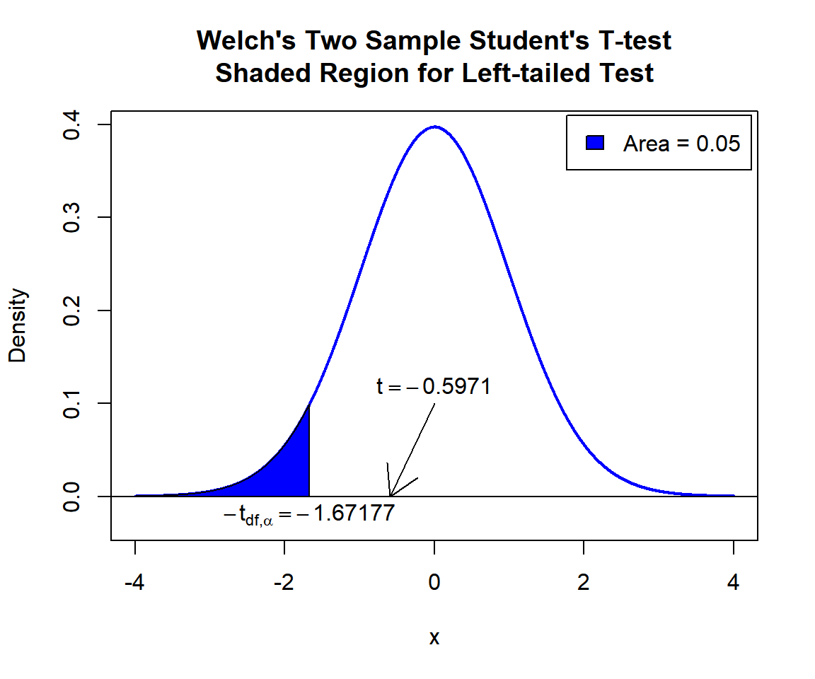
Welch’s Two Sample Student’s T-test Shaded Region for Left-tailed Test in R
6 Welch’s Two Sample T-test: Test Statistics, P-value & Degree of Freedom in R
Here for Welch’s two sample t-test, we show how to get the test
statistics (or t-value), p-values, and degrees of freedom from the
t.test() function in R, or by written code.
data_x = attitude$rating; data_y = attitude$complaints
test_object = t.test(data_x, data_y,
                     alternative = "two.sided",
                     mu = 0, conf.level = 0.9)
test_object
    Welch Two Sample t-test

data:  data_x and data_y
t = -0.5971, df = 57.54, p-value = 0.5528
alternative hypothesis: true difference in means is not equal to 0
90 percent confidence interval:
 -7.472977  3.539644
sample estimates:
mean of x mean of y
 64.63333  66.60000
To get the test statistic or t-value:
\[t = \frac{(\bar x - \bar y) - \mu_0}{\sqrt{\frac{s_x^2}{n_x} + \frac{s_y^2}{n_y}}},\]
         t
-0.5970993 [1] -0.5970993Same as:
mu = 0
sde_x = sd(data_x)^2/length(data_x)
sde_y = sd(data_y)^2/length(data_y)
SE = sqrt(sde_x + sde_y)
(mean(data_x)-mean(data_y)-mu)/SE
[1] -0.5970993To get the p-value:
Two-tailed: For positive test statistic (\(t^+\)), and negative test statistic (\(t^-\)).
\(Pvalue = 2*P(t_{df}>t^+)\) or \(Pvalue = 2*P(t_{df}<t^-)\).
One-tailed: For right-tail, \(Pvalue = P(t_{df}>t)\) or for left-tail, \(Pvalue = P(t_{df}<t)\).
[1] 0.5527835Same as:
Note that the p-value depends on the \(\text{test statistics}\) (-0.5971) and
\(\text{degrees of freedom}\) (57.54).
We also use the distribution function pt() for the
Student’s t-distribution in R.
[1] 0.552783[1] 0.552783One-tailed example:
To get the degrees of freedom:
The degrees of freedom are \(\frac{\left(\frac{s_x^2}{n_x} + \frac{s_y^2}{n_y}\right)^2}{\frac{\left(s_x^2/n_x\right)^2}{n_x-1} + \frac{\left(s_y^2/n_y\right)^2}{n_y-1}}\).
      df
57.53962 [1] 57.53962Same as:
num = ((var(data_x)/length(data_x))+(var(data_y)/length(data_y)))^2
denom1 = (((var(data_x)/length(data_x))))^2/(length(data_x)-1)
denom2 = (((var(data_y)/length(data_y))))^2/(length(data_y)-1)
num/(denom1 + denom2)
[1] 57.539627 Welch’s Two Sample T-test: Estimates, Standard Error & Confidence Interval in R
Here for Welch’s two sample t-test, we show how to get the sample
means, standard error estimate, and confidence interval from the
t.test() function in R, or by written code.
data_x = attitude$complaints; data_y = attitude$raises
test_object = t.test(data_x, data_y,
                     alternative = "two.sided",
                     mu = 0, conf.level = 0.95)
test_object
    Welch Two Sample t-test

data:  data_x and data_y
t = 0.63764, df = 54.781, p-value = 0.5264
alternative hypothesis: true difference in means is not equal to 0
95 percent confidence interval:
 -4.214941  8.148275
sample estimates:
mean of x mean of y
 66.60000  64.63333
To get the point estimates or sample means:
\[\bar x = \frac{1}{n}\sum_{i=1}^{n} x_i \;, \quad \bar y = \frac{1}{n}\sum_{i=1}^{n} y_i.\]
mean of x mean of y
66.60000 64.63333 [1] 66.60000 64.63333Same as:
[1] 66.6[1] 64.63333To get the standard error estimate:
\[\widehat {SE} = \sqrt{\frac{s_x^2}{n_x} + \frac{s_y^2}{n_y}}.\]
[1] 3.084288Same as:
[1] 3.084288To get the confidence interval for \(\mu_x - \mu_y\):
For two-tailed: \[CI = \left[(\bar x-\bar y) - t_{df, \alpha/2}*\widehat {SE} \;,\; (\bar x-\bar y) + t_{df, \alpha/2}*\widehat {SE} \right].\]
For right one-tailed: \[CI = \left[(\bar x-\bar y) - t_{df, \alpha}*\widehat {SE} \;,\; \infty \right).\]
For left one-tailed: \[CI = \left(-\infty \;,\; (\bar x-\bar y) + t_{df, \alpha}*\widehat {SE} \right].\]
[1] -4.214941  8.148275
attr(,"conf.level")
[1] 0.95[1] -4.214941 8.148275Same as:
Note that the critical values depend on the \(\alpha\) (0.05) and \(\text{degrees of freedom}\) (54.781).
alpha = 0.05; df = 54.781
SE = sqrt((var(data_x)/length(data_x))+(var(data_y)/length(data_y)))
l = (mean(data_x) - mean(data_y)) - qt(1-alpha/2, df)*SE
u = (mean(data_x) - mean(data_y)) + qt(1-alpha/2, df)*SE
c(l, u)
[1] -4.214941 8.148274One-tailed example:
The feedback form is a Google form but it does not collect any personal information.
Please click on the link below to go to the Google form.
Thank You!
Go to Feedback Form
Copyright © 2020 - 2026. All Rights Reserved by Stats Codes