One Sample T-tests in R
- 1 Test Statistic for One Sample T-test in R
- 2 Simple One Sample T-test in R
- 3 One Sample T-test Critical Value in R
- 4 Two-tailed One Sample T-test in R
- 5 One-tailed One Sample T-test in R
- 6 One Sample T-test: Test Statistics, P-value & Degree of Freedom in R
- 7 One Sample T-test: Estimate, Standard Error & Confidence Interval in R
Here, we discuss the one sample t-test in R with interpretations, including, test statistics, p-values, critical values, confidence intervals, and standard errors.
The one sample t-test in R can be performed with the
t.test() function from the base "stats" package.
The one sample t-test can be used to test whether the mean of the population where an independent random sample comes from is equal to a certain value (which is stated in the null hypothesis) or not.
In the one sample t-test, the test statistic follows a Student’s t-distribution when the null hypothesis is true.
| Question | Is the mean equal to \(\mu_0\)? | Is the mean greater than \(\mu_0\)? | Is the mean less than \(\mu_0\)? |
| Form of Test | Two-tailed | Right-tailed test | Left-tailed test |
| Null Hypothesis, \(H_0\) | \(\mu = \mu_0\) | \(\mu = \mu_0\) | \(\mu = \mu_0\) |
| Alternate Hypothesis, \(H_1\) | \(\mu \neq \mu_0\) | \(\mu > \mu_0\) | \(\mu < \mu_0\) |
Sample Steps to Run a One Sample T-test:
# Create the data for the one sample t-test

data = c(1.5, -2.0, 2.1, -2.2, 1.3, 3.2)

# Run the one sample t-test with specifications

t.test(data, alternative = "two.sided",
       mu = 0, conf.level = 0.95)
    One Sample t-test

data:  data
t = 0.71354, df = 5, p-value = 0.5074
alternative hypothesis: true mean is not equal to 0
95 percent confidence interval:
 -1.691676  2.991676
sample estimates:
mean of x
0.65 | Argument | Usage |
| x | Sample data values |
| alternative | Set alternate hypothesis as "greater", "less", or the default "two.sided" |
| mu | Population mean value in null hypothesis |
| conf.level | Level of confidence for the test and confidence interval (default = 0.95) |
Creating a One Sample T-test Object:
# Create data
data = rnorm(100)

# Create object
test_object = t.test(data, alternative = "two.sided",
                     mu = 0, conf.level = 0.95)

# Extract a component
test_object$statistic
t
0.9904068 | Test Component | Usage |
| test_object$statistic | t-statistic value |
| test_object$p.value | P-value |
| test_object$parameter | Degrees of freedom |
| test_object$estimate | Point estimate or sample mean |
| test_object$stderr | Standard error value |
| test_object$conf.int | Confidence interval |
1 Test Statistic for One Sample T-test in R
The one sample t-test has test statistics, \(t\), of the form:
\[t = \frac{\bar x - \mu_0}{s/ \sqrt n}.\] For an independent random sample that comes from a normal distribution or for large sample sizes (for example, \(n > 30\)), \(t\) is said to follow the Student’s t-distribution with \(n-1\) degrees of freedom (\(t_{n-1}\)) when the null hypothesis is true.
\(\bar x\) is the sample mean,
\(\mu_0\) is the population mean value to be tested and set in the null hypothesis,
\(s\) is the sample standard deviation, and
\(n\) is the sample size.
See also two sample t-tests (independent & unequal variance, independent & equal variance, and dependent or paired samples).
For non-parametric tests, see the sign tests for one sample and the Wilcoxon signed-rank tests for one sample.
2 Simple One Sample T-test in R
Enter the data by hand.
For the following null hypothesis \(H_0\), and alternative hypothesis \(H_1\), with the level of significance \(\alpha=0.05\).
\(H_0:\) the population mean is equal to 0 (\(\mu = 0\)).
\(H_1:\) the population mean is not equal to 0 (\(\mu \neq 0\), hence the default two-sided).
Because the level of significance is \(\alpha=0.05\), the level of confidence is \(1 - \alpha = 0.95\).
The t.test() function has the default
alternative as "two.sided", the default mean as
0, and the default level of confidence as
0.95, hence, you do not need to specify the "alternative",
"mu", and "conf.level" arguments in this case.
Or:
    One Sample t-test

data:  data
t = 1.2089, df = 14, p-value = 0.2467
alternative hypothesis: true mean is not equal to 0
95 percent confidence interval:
 -1.021951  3.661951
sample estimates:
mean of x
     1.32
The sample mean, \(\bar x\), is 1.32,
test statistic, \(t\), is 1.2089,
the degrees of freedom, \(n-1\), is 14,
the p-value, \(p\), is 0.2467,
the 95% confidence interval is [-1.021951, 3.661951].
Interpretation:
P-value: With the p-value (\(p = 0.2467\)) being greater than the level of significance 0.05, we fail to reject the null hypothesis that the population mean is equal to 0.
\(t\)-statistic: With test statistics value (\(t = 1.2089\)) being between the two critical values, \(-t_{n-1, \alpha/2}=\text{qt(0.025, 14)}=-2.1447867\) and \(t_{n-1, \alpha/2}=\text{qt(0.975, 14)}=2.1447867\) (or not in the shaded region), we fail to reject the null hypothesis that the population mean is equal to 0.
Confidence Interval: With the null hypothesis mean value (\(\mu = 0\)) being inside the confidence interval, \([-1.021951, 3.661951]\), we fail to reject the null hypothesis that the population mean is equal to 0.
x = seq(-4, 4, 1/1000); y = dt(x, df=14)
plot(x, y, type = "l",
     xlim = c(-4, 4), ylim = c(-0.03, max(y)),
     main = "One Sample Student's T-test
Shaded Region for Simple T-test",
     xlab = "x", ylab = "Density",
     lwd = 2, col = "blue")
abline(h=0)
# Add shaded region and legend
point1 = qt(0.025, 14); point2 = qt(0.975, 14)
polygon(x = c(-4, x[x <= point1], point1),
        y = c(0, y[x <= point1], 0),
        col = "blue")
polygon(x = c(x[x >= point2], 4, point2),
        y = c(y[x >= point2], 0, 0),
        col = "blue")
legend("topright", c("Area = 0.05"),
       fill = c("blue"), inset = 0.01)
# Add critical value and t-value
arrows(0, 0.1, 1.2089, 0)
text(0, 0.12, "t = 1.2089")
text(-2.144787, -0.02, expression(-t[n-1][','][alpha/2]==-2.144787))
text(2.144787, -0.02, expression(t[n-1][','][alpha/2]==2.144787))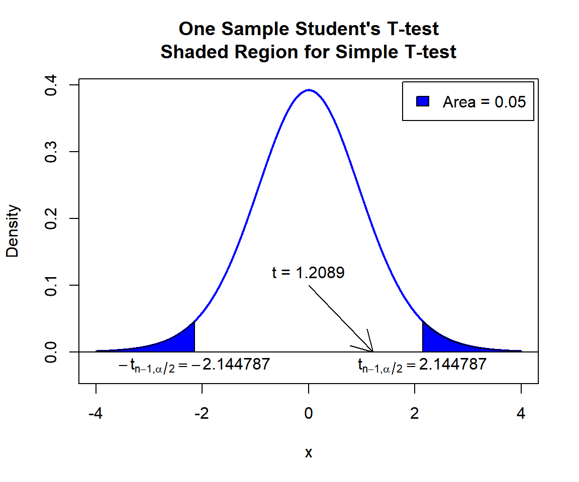
One Sample Student’s T-test Shaded Region for Simple T-test in R
See line charts, shading areas under a curve, lines & arrows on plots, mathematical expressions on plots, and legends on plots for more details on making the plot above.
3 One Sample T-test Critical Value in R
To get the critical value for a one sample t-test in R, you can use
the qt() function for Student’s t-distribution to derive
the quantile associated with the given level of significance value \(\alpha\).
For two-tailed test with level of significance \(\alpha\). The critical values are: qt(\(\alpha/2\), df) and qt(\(1-\alpha/2\), df).
For one-tailed test with level of significance \(\alpha\). The critical value is: for left-tailed, qt(\(\alpha\), df); and for right-tailed, qt(\(1-\alpha\), df).
Example:
For \(\alpha = 0.05\), and \(\text{df = 59}\).
Two-tailed:
[1] -2.000995[1] 2.000995One-tailed:
[1] -1.671093[1] 1.6710934 Two-tailed One Sample T-test in R
Using the trees$Height data from the "datasets" package with 10 sample observations from 31 observations below:
[1] 70 83 75 76 74 85 74 82 80 87For the following null hypothesis \(H_0\), and alternative hypothesis \(H_1\), with the level of significance \(\alpha=0.1\).
\(H_0:\) the population mean is equal to 79 (\(\mu = 79\)).
\(H_1:\) the population mean is not equal to 79 (\(\mu \neq 79\), hence the default two-sided).
Because the level of significance is \(\alpha=0.1\), the level of confidence is \(1 - \alpha = 0.9\).
    One Sample t-test

data:  trees$Height
t = -2.6214, df = 30, p-value = 0.01362
alternative hypothesis: true mean is not equal to 79
90 percent confidence interval:
 74.05764 77.94236
sample estimates:
mean of x
       76
Interpretation:
P-value: With the p-value (\(p = 0.01362\)) being lower than the level of significance 0.1, we reject the null hypothesis that the population mean is equal to 79.
\(t\)-statistic: With test statistics value (\(t = -2.6214\)) being in the critical region (shaded area), that is, \(t = -2.6214\) less than \(-t_{n-1, \alpha/2}=\text{qt(0.05, 30)}=-1.6972609\), we reject the null hypothesis that the population mean is equal to 79.
Confidence Interval: With the null hypothesis mean value (\(\mu = 79\)) being outside the confidence interval, \([74.05764, 77.94236]\), we reject the null hypothesis that the population mean is equal to 79.
x = seq(-4, 4, 1/1000); y = dt(x, df=30)
plot(x, y, type = "l",
     xlim = c(-4, 4), ylim = c(-0.03, max(y)),
     main = "One Sample Student's T-test
Shaded Region for Two-tailed Test",
     xlab = "x", ylab = "Density",
     lwd = 2, col = "blue")
abline(h=0)
# Add shaded region and legend
point1 = qt(0.05, 30); point2 = qt(0.95, 30)
polygon(x = c(-4, x[x <= point1], point1),
        y = c(0, y[x <= point1], 0),
        col = "blue")
polygon(x = c(x[x >= point2], 4, point2),
        y = c(y[x >= point2], 0, 0),
        col = "blue")
legend("topright", c("Area = 0.1"),
       fill = c("blue"), inset = 0.01)
# Add critical value and t-value
arrows(-2.6214, 0.1, -2.6214, 0)
text(-2.6214, 0.12, expression(t==-2.6214))
text(-1.697261, -0.02, expression(-t[n-1][','][alpha/2]==-1.697261))
text(1.697261, -0.02, expression(t[n-1][','][alpha/2]==1.697261))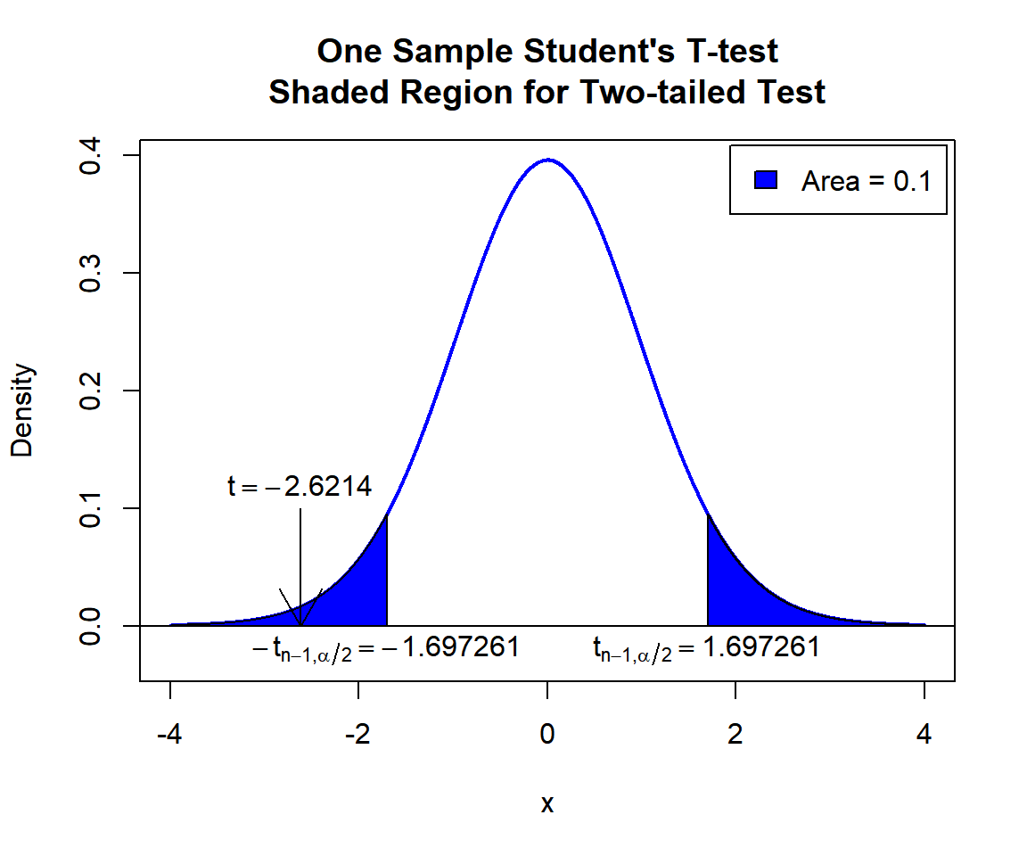
One Sample Student’s T-test Shaded Region for Two-tailed Test in R
5 One-tailed One Sample T-test in R
Right Tailed Test
Using the trees$Height data from the "datasets" package with 10 sample observations from 31 observations below:
[1] 70 72 79 76 75 74 71 64 74 87For the following null hypothesis \(H_0\), and alternative hypothesis \(H_1\), with the level of significance \(\alpha=0.05\).
\(H_0:\) the population mean is equal to 72.5 (\(\mu = 72.5\)).
\(H_1:\) the population mean is greater than 72.5 (\(\mu > 72.5\), hence one-sided).
Because the level of significance is \(\alpha=0.05\), the level of confidence is \(1 - \alpha = 0.95\).
    One Sample t-test

data:  trees$Height
t = 3.0583, df = 30, p-value = 0.002326
alternative hypothesis: true mean is greater than 72.5
95 percent confidence interval:
 74.05764      Inf
sample estimates:
mean of x
       76
Interpretation:
P-value: With the p-value (\(p = 0.002326\)) being lower than the level of significance 0.05, we reject the null hypothesis that the population mean is equal to 72.5.
\(t\)-statistic: With test statistics value (\(t = 3.0583\)) being in the critical region (shaded area), that is, \(t = 3.0583\) greater than \(t_{n-1, \alpha}=\text{qt(0.95, 30)}=1.6972609\), we reject the null hypothesis that the population mean is equal to 72.5.
Confidence Interval: With the null hypothesis mean value (\(\mu = 72.5\)) being outside the confidence interval, \([74.05764, \infty)\), we reject the null hypothesis that the population mean is equal to 72.5.
x = seq(-4, 4, 1/1000); y = dt(x, df=30)
plot(x, y, type = "l",
     xlim = c(-4, 4), ylim = c(-0.03, max(y)),
     main = "One Sample Student's T-test
Shaded Region for Right-tailed Test",
     xlab = "x", ylab = "Density",
     lwd = 2, col = "blue")
abline(h=0)
# Add shaded region and legend
point = qt(0.95, 30)
polygon(x = c(x[x >= point], 4, point),
        y = c(y[x >= point], 0, 0),
        col = "blue")
legend("topright", c("Area = 0.05"),
       fill = c("blue"), inset = 0.01)
# Add critical value and t-value
arrows(3.0583, 0.1, 3.0583, 0)
text(3.0583, 0.12, expression(t==3.0583))
text(1.697261, -0.02, expression(t[n-1][','][alpha]==1.697261))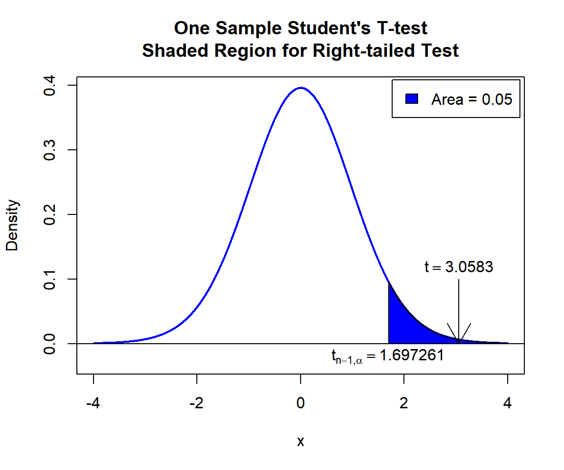
One Sample Student’s T-test Shaded Region for Right-tailed Test in R
Left Tailed Test
For the following null hypothesis \(H_0\), and alternative hypothesis \(H_1\), with the level of significance \(\alpha=0.1\).
\(H_0:\) the population mean is equal to 77 (\(\mu = 77\)).
\(H_1:\) the population mean is less than 77 (\(\mu < 77\), hence one-sided).
Because the level of significance is \(\alpha=0.1\), the level of confidence is \(1 - \alpha = 0.9\).
    One Sample t-test

data:  trees$Height
t = -0.87381, df = 30, p-value = 0.1946
alternative hypothesis: true mean is less than 77
90 percent confidence interval:
     -Inf 77.49965
sample estimates:
mean of x
       76
Interpretation:
P-value: With the p-value (\(p = 0.1946\)) being greater than the level of significance 0.1, we fail to reject the null hypothesis that the population mean is equal to 77.
\(t\)-statistic: With test statistics value (\(t = -0.87381\)) being greater than the critical value (not in the shaded region), that is, \(t = -0.87381\) greater than \(-t_{n-1, \alpha}=\text{qt(0.1, 30)}=-1.310415\), we fail to reject the null hypothesis that the population mean is equal to 77.
Confidence Interval: With the null hypothesis mean value (\(\mu = 77\)) being inside the confidence interval, \((-\infty, 77.49965]\), we fail to reject the null hypothesis that the population mean is equal to 77.
x = seq(-4, 4, 1/1000); y = dt(x, df=30)
plot(x, y, type = "l",
     xlim = c(-4, 4), ylim = c(-0.03, max(y)),
     main = "One Sample Student's T-test
Shaded Region for Left-tailed Test",
     xlab = "x", ylab = "Density",
     lwd = 2, col = "blue")
abline(h=0)
# Add shaded region and legend
point = qt(0.1, 30)
polygon(x = c(-4, x[x <= point], point),
        y = c(0, y[x <= point], 0),
        col = "blue")
legend("topright", c("Area = 0.1"),
       fill = c("blue"), inset = 0.01)
# Add critical value and t-value
arrows(0, 0.1, -0.87381, 0)
text(0, 0.12, expression(t==-0.87381))
text(-1.310415, -0.03, expression(-t[n-1][','][alpha]==-1.310415))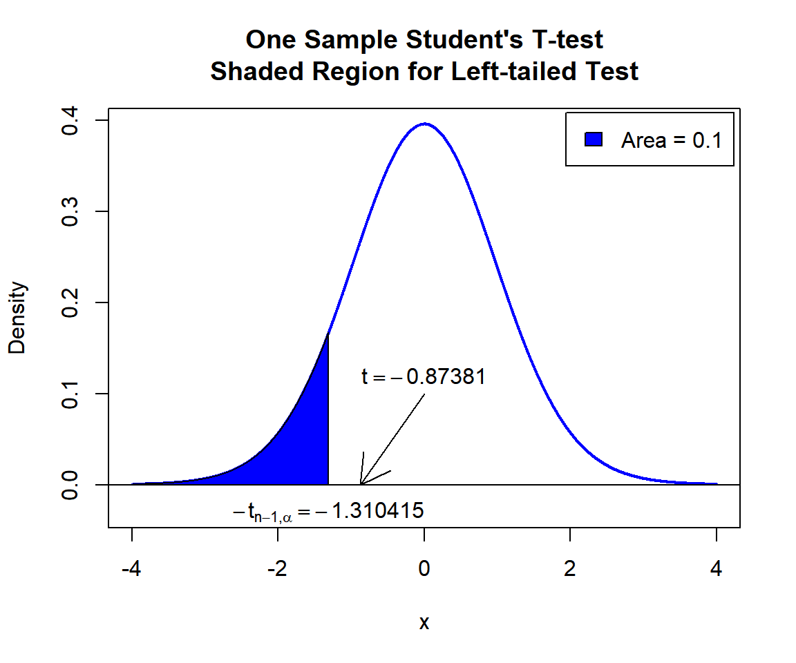
One Sample Student’s T-test Shaded Region for Left-tailed Test in R
6 One Sample T-test: Test Statistics, P-value & Degree of Freedom in R
Here for a one sample t-test, we show how to get the test statistics
(or t-value), p-values, and degrees of freedom from the
t.test() function in R, or by written code.
data_os = trees$Height
test_object = t.test(data_os, alternative = "two.sided",
                     mu = 75, conf.level = 0.95)
test_object
    One Sample t-test

data:  data_os
t = 0.87381, df = 30, p-value = 0.3892
alternative hypothesis: true mean is not equal to 75
95 percent confidence interval:
 73.6628 78.3372
sample estimates:
mean of x
       76
To get the test statistic or t-value:
\[t = \frac{\bar x - \mu_0}{s/ \sqrt n}.\]
        t
0.8738116 [1] 0.8738116Same as:
[1] 0.8738116To get the p-value:
Two-tailed: For positive test statistic (\(t^+\)), and negative test statistic (\(t^-\)).
\(Pvalue = 2*P(t_{n-1}>t^+)\) or \(Pvalue = 2*P(t_{n-1}<t^-)\).
One-tailed: For right-tail, \(Pvalue = P(t_{n-1}>t)\) or for left-tail, \(Pvalue = P(t_{n-1}<t)\).
[1] 0.3891622Same as:
Note that the p-value depends on the \(\text{test statistics}\) (0.8738116) and
\(\text{degrees of freedom}\) (30). We
also use the distribution function pt() for the Student’s
t-distribution in R.
[1] 0.3891623[1] 0.3891623One-tailed example:
To get the degrees of freedom:
The degrees of freedom are \(n - 1\).
df
30 [1] 30Same as:
[1] 307 One Sample T-test: Estimate, Standard Error & Confidence Interval in R
Here for a one sample t-test, we show how to get the sample mean,
standard error estimate, and confidence interval from the
t.test() function in R, or by written code.
data_os = trees$Height
test_object = t.test(data_os, alternative = "two.sided",
                     mu = 74, conf.level = 0.9)
test_object
    One Sample t-test

data:  data_os
t = 1.7476, df = 30, p-value = 0.09076
alternative hypothesis: true mean is not equal to 74
90 percent confidence interval:
 74.05764 77.94236
sample estimates:
mean of x
       76
To get the point estimate or sample mean:
\[\bar x = \frac{1}{n}\sum_{i=1}^{n} x_i.\]
mean of x
76 [1] 76Same as:
[1] 76To get the standard error estimate (or sample standard deviation divide by square root of \(n\)):
\[\widehat {SE} = \frac{s}{\sqrt n} = \sqrt {\frac{1}{n(n-1)}\sum_{i=1}^{n} (x_i-\bar x)^2}.\]
[1] 1.144411Same as:
Or:
[1] 1.144411To get the confidence interval for \(\mu\):
For two-tailed: \[CI = \left[\bar x - t_{n-1, \alpha/2}*\frac{s}{\sqrt n} \;,\; \bar x + t_{n-1, \alpha/2}*\frac{s}{\sqrt n} \right].\]
For right one-tailed: \[CI = \left[\bar x - t_{n-1, \alpha}*\frac{s}{\sqrt n} \;,\; \infty \right).\]
For left one-tailed: \[CI = \left(-\infty \;,\; \bar x + t_{n-1, \alpha}*\frac{s}{\sqrt n} \right].\]
[1] 74.05764 77.94236
attr(,"conf.level")
[1] 0.9[1] 74.05764 77.94236Same as:
Note that the critical values depend on the \(\alpha\) (0.1) and \(\text{degrees of freedom}\) (30).
alpha = 0.1; df = length(data_os)-1
SE = sd(data_os)/sqrt(length(data_os))
l = mean(data_os) - qt(1-alpha/2, df)*SE
u = mean(data_os) + qt(1-alpha/2, df)*SE
c(l, u)
[1] 74.05764 77.94236One-tailed example:
The feedback form is a Google form but it does not collect any personal information.
Please click on the link below to go to the Google form.
Thank You!
Go to Feedback Form
Copyright © 2020 - 2026. All Rights Reserved by Stats Codes