Pearson’s Correlation Coefficient Tests in R
- 1 Test Statistic for Pearson’s Correlation Coefficient Test in R
- 2 Simple Pearson’s Correlation Coefficient Test in R
- 3 Pearson’s Correlation Coefficient Test Critical Value in R
- 4 Two-tailed Pearson’s Correlation Coefficient Test in R
- 5 One-tailed Pearson’s Correlation Coefficient Test in R
- 6 Pearson’s Correlation Coefficient Test: Test Statistics, P-value & Degree of Freedom in R
- 7 Pearson’s Correlation Coefficient Test: Estimate & Confidence Interval in R
Here, we discuss the Pearson’s correlation coefficient test in R with interpretations, including, test statistics, p-values, critical values, and confidence intervals.
The Pearson’s correlation coefficient test in R can be performed with
the cor.test() function from the base "stats" package.
The Pearson’s correlation coefficient test can be used to test whether there is a linear correlation between two variables, or if there is none as stated in the null hypothesis.
In the Pearson’s correlation coefficient test, the test statistic follows a Student’s t-distribution when the null hypothesis is true.
| Question | Is there a linear correlation between x and y? | Is there a positive linear correlation between x and y? | Is there a negative linear correlation between x and y? |
| Form of Test | Two-tailed | Right-tailed test | Left-tailed test |
| Null Hypothesis, \(H_0\) | \(\rho = 0\) | \(\rho = 0\) | \(\rho = 0\) |
| Alternate Hypothesis, \(H_1\) | \(\rho \neq 0\) | \(\rho > 0\) | \(\rho < 0\) |
Sample Steps to Run a Pearson’s Correlation Coefficient Test:
# Create the data samples for the Pearson's correlation coefficient test
# Values are paired based on matching position in each sample

data_x = c(8.3, 11.8, 11.2, 10.7, 9.8)
data_y = c(9.4, 10.0, 8.0, 13.3, 8.7)

# Run the Pearson's correlation coefficient test with specifications

cor.test(data_x, data_y, method = "pearson",
         alternative = "two.sided",
         conf.level = 0.95)
    Pearson's product-moment correlation

data:  data_x and data_y
t = 0.21894, df = 3, p-value = 0.8407
alternative hypothesis: true correlation is not equal to 0
95 percent confidence interval:
 -0.8510185  0.9072886
sample estimates:
      cor
0.1254056 | Argument | Usage |
| x, y | The two sample data values |
| alternative | Set alternate hypothesis as "greater", "less", or the default "two.sided" |
| method | Set to "pearson", the default is "pearson" |
| conf.level | Level of confidence for the test and confidence interval (default = 0.95) |
Creating a Pearson’s Correlation Coefficient Test Object:
# Create data
data_x = rnorm(40); data_y = rnorm(40)

# Create object
cor_object = cor.test(data_x, data_y, method = "pearson",
                      alternative = "two.sided",
                      conf.level = 0.95)

# Extract a component
cor_object$statistic
t
0.3225507 | Test Component | Usage |
| cor_object$statistic | Test-statistic value |
| cor_object$p.value | P-value |
| cor_object$parameter | Degrees of freedom |
| cor_object$estimate | Sample correlation coefficient |
| cor_object$conf.int | Confidence interval |
1 Test Statistic for Pearson’s Correlation Coefficient Test in R
The Pearson’s correlation coefficient test has test statistics, \(t\), of the form:
\[t = \frac{r}{\sqrt{\frac{1 - r^2}{n-2}}},\]
where the sample Pearson’s correlation coefficient,
\[ r = \frac{n\sum ^n _{i=1} x_i y_i - \sum ^n _{i=1} x_i\sum ^n _{i=1} y_i} {\sqrt{n\sum ^n _{i=1} x_i^2-\left(\sum ^n _{i=1} x_i\right)^2}~\sqrt{n\sum ^n _{i=1} y_i^2-\left(\sum ^n _{i=1} y_i\right)^2}}\]
or \[r = \frac{\sum ^n _{i=1}(x_i - \bar{x})(y_i - \bar{y})}{\sqrt{\sum ^n _{i=1}(x_i - \bar{x})^2} \sqrt{\sum ^n _{i=1}(y_i - \bar{y})^2}}\]
For an independent random sample of matched pairs that come from normal distributions, \(t\) is said to follow the Student’s t-distribution with \(n-2\) degrees of freedom (\(t_{n-2}\)) when the null hypothesis is true.
\(\sum\) is the summation sign,
\(x_i's\), and \(y_i's\) are the sample data values,
\(\bar x\) is the sample mean of the \(x_i's\), \(\bar y\) is the sample mean of the \(y_i's\), and
\(n \in \{3, 4, 5 ...\}\) is the number of pairs in the sample.
For a non-parametric test, see the Spearman’s rank correlation coefficient test.
2 Simple Pearson’s Correlation Coefficient Test in R
Enter the data by hand.
data_x = c(10.5, 10.5, 10.4, 9.7, 8.1,
           10.6, 11.7, 9.2, 8.7, 9.9)
data_y = c(10.7, 10.2, 10.7, 9.5, 8.9,
           10.4, 10.5, 9.7, 9.6, 8.8)
Check for linear relationship or absence of non-linear relationship before testing.
plot(data_x, data_y,
     main = "X vs Y",
     xlab = "X Variable",
     ylab = "Y Variable")
# Add line
abline(lm(data_y ~ data_x))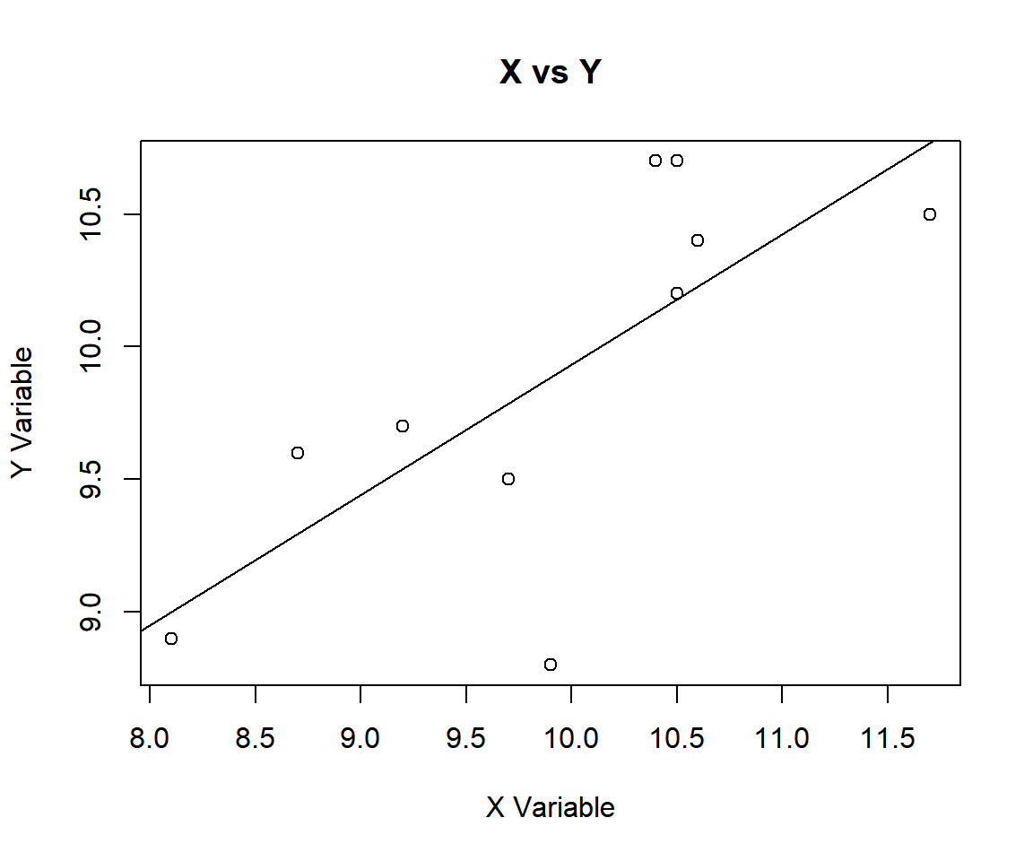
Pearson’s Correlation Coefficient Test X vs Y in R
For the following null hypothesis \(H_0\), and alternative hypothesis \(H_1\), with the level of significance \(\alpha=0.05\).
\(H_0:\) there is no linear relationship between \(x\) and \(y\) (\(\rho = 0\)).
\(H_1:\) there is a linear relationship between \(x\) and \(y\) (\(\rho \neq 0\), hence the default two-sided).
Because the level of significance is \(\alpha=0.05\), the level of confidence is \(1 - \alpha = 0.95\).
The cor.test() function has the default
alternative as "two.sided", the default method as
"pearson", and the default level of confidence as
0.95, hence, you do not need to specify the "alternative",
"method” and "conf.level" arguments in this case.
Or:
    Pearson's product-moment correlation

data:  data_x and data_y
t = 3.032, df = 8, p-value = 0.01626
alternative hypothesis: true correlation is not equal to 0
95 percent confidence interval:
 0.1882826 0.9318353
sample estimates:
     cor
0.731224
The sample correlation coefficient, \(r\), is 0.731224,
test statistic, \(t\), is 3.032,
the degrees of freedom, \(n-2\), is 8,
the p-value, \(p\), is 0.01626,
the 95% confidence interval is [0.1882826, 0.9318353].
Interpretation:
Note that for cor.test() in R, the Pearson’s correlation
test’s p-value and T-statistic methods may disagree with the confidence
interval method for some edge cases. This is because the p-value and
T-statistic are based on the Student’s t-distribution, while the
confidence interval is based on the Fisher
transformations.
P-value: With the p-value (\(p = 0.01626\)) being less than the level of significance 0.05, we reject the null hypothesis that the population correlation coefficient is equal to 0.
\(t\)-statistic: With test statistics value (\(t = 3.032\)) being in the critical region (shaded area), that is, \(t = 3.032\) greater than \(t_{n-2,\alpha/2}=\text{qt(0.975, 8)}=2.3060041\), we reject the null hypothesis that the population correlation coefficient is equal to 0.
Confidence Interval: With the null hypothesis population correlation coefficient (\(\rho = 0\)) being outside the confidence interval, \([0.1882826, 0.9318353]\), we reject the null hypothesis that the population correlation coefficient is equal to 0.
x = seq(-4, 4, 1/1000); y = dt(x, df=8)
plot(x, y, type = "l",
     xlim = c(-4, 4), ylim = c(-0.03, max(y)),
     main = "Pearson's Correlation Coefficient Test
Shaded Region for Simple Correlation Test",
     xlab = "x", ylab = "Density",
     lwd = 2, col = "blue")
abline(h=0)
# Add shaded region and legend
point1 = qt(0.025, 8); point2 = qt(0.975, 8)
polygon(x = c(-4, x[x <= point1], point1),
        y = c(0, y[x <= point1], 0),
        col = "blue")
polygon(x = c(x[x >= point2], 4, point2),
        y = c(y[x >= point2], 0, 0),
        col = "blue")
legend("topright", c("Area = 0.05"),
       fill = c("blue"), inset = 0.01)
# Add critical value and t-value
arrows(3.032, 0.1, 3.032, 0)
text(3.032, 0.12, "t = 3.032")
text(-2.306004, -0.02, expression(-t[n-2][','][alpha/2]==-2.306004))
text(2.306004, -0.02, expression(t[n-2][','][alpha/2]==2.306004))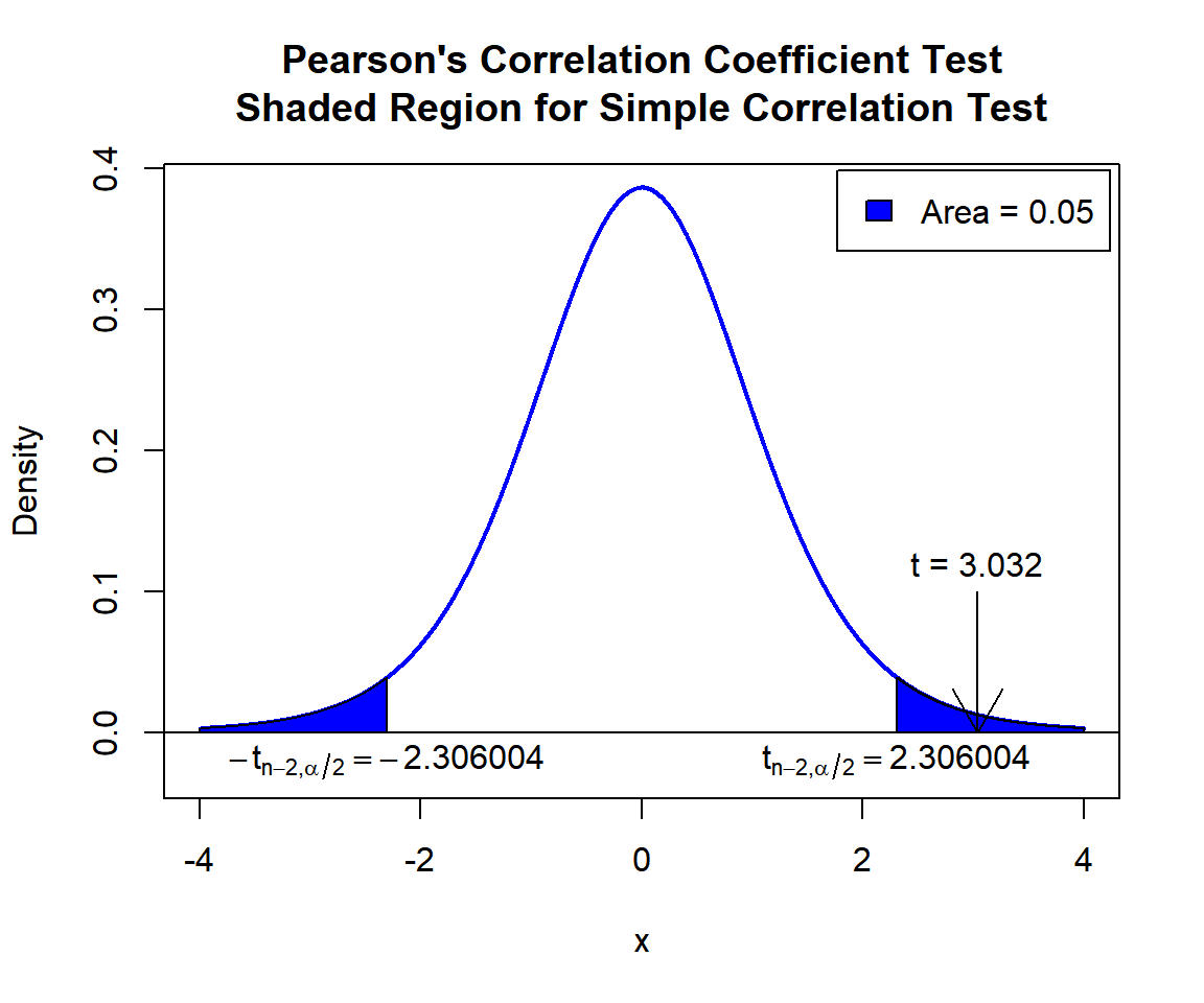
Pearson’s Correlation Coefficient Test Shaded Region for Simple Correlation Test in R
See line charts, shading areas under a curve, lines & arrows on plots, mathematical expressions on plots, and legends on plots for more details on making the plot above.
3 Pearson’s Correlation Coefficient Test Critical Value in R
To get the critical value for a Pearson’s correlation coefficient
test in R, you can use the qt() function for Student’s
t-distribution to derive the quantile associated with the given level of
significance value \(\alpha\).
For two-tailed test with level of significance \(\alpha\). The critical values are: qt(\(\alpha/2\), df) and qt(\(1-\alpha/2\), df).
For one-tailed test with level of significance \(\alpha\). The critical value is: for left-tailed, qt(\(\alpha\), df); and for right-tailed, qt(\(1-\alpha\), df).
Example:
For \(\alpha = 0.1\), and \(\text{df = n-2=24}\)
Two-tailed:
[1] -1.710882[1] 1.710882One-tailed:
[1] -1.317836[1] 1.3178364 Two-tailed Pearson’s Correlation Coefficient Test in R
Using the swiss data from the "datasets" package with 10 sample observations from 47 rows below:
   Fertility Agriculture Examination Education Catholic Infant.Mortality
1       80.2        17.0          15        12     9.96             22.2
6       76.1        35.3           9         7    90.57             26.6
10      82.9        45.2          16        13    91.38             24.4
17      71.7        34.0          17         8     3.30             20.0
23      56.6        50.9          22        12    15.14             16.7
29      58.3        26.8          25        19    18.46             20.9
38      79.3        63.1          13        13    96.83             18.1
39      70.4        38.4          26        12     5.62             20.3
45      35.0         1.2          37        53    42.34             18.0
47      42.8        27.7          22        29    58.33             19.3
For “Infant.Mortality” as the \(x\) group versus “Agriculture” as the \(y\) group.
For the following null hypothesis \(H_0\), and alternative hypothesis \(H_1\), with the level of significance \(\alpha=0.1\).
\(H_0:\) there is no linear relationship between \(x\) and \(y\) (\(\rho = 0\)).
\(H_1:\) there is a linear relationship between \(x\) and \(y\) (\(\rho \neq 0\), hence the default two-sided).
Because the level of significance is \(\alpha=0.1\), the level of confidence is \(1 - \alpha = 0.9\).
cor.test(swiss$Infant.Mortality, swiss$Agriculture,
         method = "pearson",
         alternative = "two.sided",
         conf.level = 0.9)
    Pearson's product-moment correlation

data:  swiss$Infant.Mortality and swiss$Agriculture
t = -0.40901, df = 45, p-value = 0.6845
alternative hypothesis: true correlation is not equal to 0
90 percent confidence interval:
 -0.2994405  0.1848862
sample estimates:
        cor
-0.06085861
Interpretation:
P-value: With the p-value (\(p = 0.6845\)) being greater than the level of significance 0.1, we fail to reject the null hypothesis that the population correlation coefficient is equal to 0.
\(t\)-statistic: With test statistics value (\(t = -0.40901\)) being between the two critical values, \(-t_{n-2,\alpha/2}=\text{qt(0.05, 45)}=-1.6794274\) and \(t_{n-2,\alpha/2}=\text{qt(0.95, 45)}=1.6794274\) (or not in the shaded region), we fail to reject the null hypothesis that the population correlation coefficient is equal to 0.
Confidence Interval: With the null hypothesis correlation coefficient value (\(\rho = 0\)) being inside the confidence interval, \([-0.2994405, 0.1848862]\), we fail to reject the null hypothesis that the population correlation coefficient is equal to 0.
x = seq(-4, 4, 1/1000); y = dt(x, df=45)
plot(x, y, type = "l",
     xlim = c(-4, 4), ylim = c(-0.03, max(y)),
     main = "Pearson's Correlation Coefficient Test
Shaded Region for Two-tailed Test",
     xlab = "x", ylab = "Density",
     lwd = 2, col = "blue")
abline(h=0)
# Add shaded region and legend
point1 = qt(0.05, 45); point2 = qt(0.95, 45)
polygon(x = c(-4, x[x <= point1], point1),
        y = c(0, y[x <= point1], 0),
        col = "blue")
polygon(x = c(x[x >= point2], 4, point2),
        y = c(y[x >= point2], 0, 0),
        col = "blue")
legend("topright", c("Area = 0.1"),
       fill = c("blue"), inset = 0.01)
# Add critical value and t-value
arrows(0, 0.1, -0.40901, 0)
text(0, 0.12, expression(t==-0.40901))
text(-1.679427, -0.02, expression(-t[n-2][','][alpha/2]==-1.679427))
text(1.679427, -0.02, expression(t[n-2][','][alpha/2]==1.679427))
Pearson’s Correlation Coefficient Test Shaded Region for Two-tailed Test in R
5 One-tailed Pearson’s Correlation Coefficient Test in R
Right Tailed Test
Using the swiss data from the "datasets" package above.
For “Examination” as the \(x\) group versus “Education” as the \(y\) group.
For the following null hypothesis \(H_0\), and alternative hypothesis \(H_1\), with the level of significance \(\alpha=0.05\).
\(H_0:\) there is no linear relationship between \(x\) and \(y\) (\(\rho = 0\)).
\(H_1:\) there is a positive linear relationship between \(x\) and \(y\) (\(\rho > 0\), hence one-sided).
Because the level of significance is \(\alpha=0.05\), the level of confidence is \(1 - \alpha = 0.95\).
cor.test(swiss$Examination, swiss$Education,
         method = "pearson",
         alternative = "greater",
         conf.level = 0.95)
    Pearson's product-moment correlation

data:  swiss$Examination and swiss$Education
t = 6.5463, df = 45, p-value = 2.406e-08
alternative hypothesis: true correlation is greater than 0
95 percent confidence interval:
 0.548497 1.000000
sample estimates:
      cor
0.6984153
Interpretation:
P-value: With the p-value (\(p = 2.406e-08\)) being less than the level of significance 0.05, we reject the null hypothesis that the population correlation coefficient is equal to 0.
\(t\)-statistic: With test statistics value (\(t = 6.5463\)) being in the critical region (shaded area), that is, \(t = 6.5463\) greater than \(t_{n-2,\alpha}=\text{qt(0.95, 45)}=1.6794274\), we reject the null hypothesis that the population correlation coefficient is equal to 0.
Confidence Interval: With the null hypothesis population correlation coefficient value (\(\rho = 0\)) being outside the confidence interval, \([0.548497, 1.0)\), we reject the null hypothesis that the population correlation coefficient is equal to 0.
x = seq(-7, 7, 1/1000); y = dt(x, df=45)
plot(x, y, type = "l",
     xlim = c(-7, 7), ylim = c(-0.03, max(y)),
     main = "Pearson's Correlation Coefficient Test
Shaded Region for Right-tailed Test",
     xlab = "x", ylab = "Density",
     lwd = 2, col = "blue")
abline(h=0)
# Add shaded region and legend
point = qt(0.95, 45)
polygon(x = c(x[x >= point], 7, point),
        y = c(y[x >= point], 0, 0),
        col = "blue")
legend("topright", c("Area = 0.05"),
       fill = c("blue"), inset = 0.01)
# Add critical value and t-value
arrows(6.5463, 0.1, 6.5463, 0)
text(6.5463, 0.12, expression(t==6.5463))
text(1.679427, -0.02, expression(t[n-2][','][alpha]==1.679427))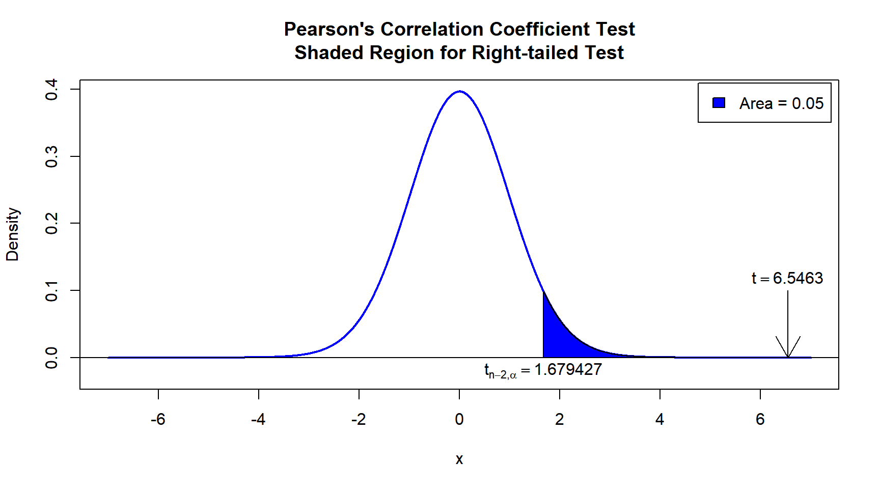
Pearson’s Correlation Coefficient Test Shaded Region for Right-tailed Test in R
Left Tailed Test
Using the swiss data from the "datasets" package above.
For “Education” as the \(x\) group versus “Infant.Mortality” as the \(y\) group.
For the following null hypothesis \(H_0\), and alternative hypothesis \(H_1\), with the level of significance \(\alpha=0.1\).
\(H_0:\) there is no linear relationship between \(x\) and \(y\) (\(\rho = 0\)).
\(H_1:\) there is a negative linear relationship between \(x\) and \(y\) (\(\rho < 0\), hence one-sided).
Because the level of significance is \(\alpha=0.1\), the level of confidence is \(1 - \alpha = 0.9\).
cor.test(swiss$Education, swiss$Infant.Mortality,
         method = "pearson",
         alternative = "less", conf.level = 0.9)
    Pearson's product-moment correlation

data:  swiss$Education and swiss$Infant.Mortality
t = -0.66958, df = 45, p-value = 0.2533
alternative hypothesis: true correlation is less than 0
90 percent confidence interval:
 -1.00000000  0.09327882
sample estimates:
        cor
-0.09932185
Interpretation:
P-value: With the p-value (\(p = 0.2533\)) being greater than the level of significance 0.1, we fail to reject the null hypothesis that the population correlation coefficient is equal to 0.
\(t\)-statistic: With test statistics value (\(t = -0.66958\)) being greater than the critical value (not in the shaded region), that is, \(t = -0.66958\) greater than \(-t_{n-2,\alpha}=\text{qt(0.1, 45)}=-1.3006493\), we fail to reject the null hypothesis that the population correlation coefficient is equal to 0.
Confidence Interval: With the null hypothesis population correlation coefficient value (\(\rho = 0\)) being inside the confidence interval, \((-1.0, 0.09327882]\), we fail to reject the null hypothesis that the population correlation coefficient is equal to 0.
x = seq(-4, 4, 1/1000); y = dt(x, df=45)
plot(x, y, type = "l",
     xlim = c(-4, 4), ylim = c(-0.03, max(y)),
     main = "Pearson's Correlation Coefficient Test
Shaded Region for Left-tailed Test",
     xlab = "x", ylab = "Density",
     lwd = 2, col = "blue")
abline(h=0)
# Add shaded region and legend
point = qt(0.1, 45)
polygon(x = c(-4, x[x <= point], point),
        y = c(0, y[x <= point], 0),
        col = "blue")
legend("topright", c("Area = 0.1"),
       fill = c("blue"), inset = 0.01)
# Add critical value and t-value
arrows(0, 0.1, -0.66958, 0)
text(0, 0.12, expression(t==-0.66958))
text(-1.300649, -0.03, expression(-t[n-2][','][alpha]==-1.300649))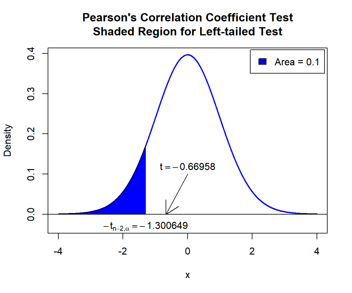
Pearson’s Correlation Coefficient Test Shaded Region for Left-tailed Test in R
6 Pearson’s Correlation Coefficient Test: Test Statistics, P-value & Degree of Freedom in R
Here for a Pearson’s correlation coefficient test, we show how to get
the test statistics (or t-value), p-values, and degrees of freedom from
the cor.test() function in R, or by written code.
data_x = swiss$Fertility; data_y = swiss$Infant.Mortality
cor_object = cor.test(data_x, data_y,
                      method = "pearson",
                      alternative = "two.sided",
                      conf.level = 0.95)
cor_object
    Pearson's product-moment correlation

data:  data_x and data_y
t = 3.0737, df = 45, p-value = 0.003585
alternative hypothesis: true correlation is not equal to 0
95 percent confidence interval:
 0.1469699 0.6285366
sample estimates:
     cor
0.416556
To get the test statistic or t-value:
\[t = \frac{r}{\sqrt{\frac{1 - r^2}{n-2}}},\]
where the correlation coefficient \[r = \frac{n\sum x_i y_i - \sum x_i\sum y_i} {\sqrt{n\sum x_i^2-\left(\sum x_i\right)^2}~\sqrt{n\sum y_i^2-\left(\sum y_i\right)^2}}\]
       t
3.073712 [1] 3.073712Same as:
n = length(data_x)
num = n*sum(data_x*data_y)-sum(data_x)*sum(data_y)
denom1 = sqrt(n*sum(data_x^2)-(sum(data_x)^2))
denom2 = sqrt(n*sum(data_y^2)-(sum(data_y)^2))
r = num/(denom1*denom2)
t = r/(sqrt((1-r^2)/(n-2)))
t
[1] 3.073712To get the p-value:
Two-tailed: For positive test statistic (\(t^+\)), and negative test statistic (\(t^-\)).
\(Pvalue = 2*P(t_{n-2}>t^+)\) or \(Pvalue = 2*P(t_{n-2}<t^-)\).
One-tailed: For right-tail, \(Pvalue = P(t_{n-2}>t)\) or for left-tail, \(Pvalue = P(t_{n-2}<t)\).
[1] 0.003585238Same as:
Note that the p-value depends on the \(\text{test statistics}\) (3.073712) and
\(\text{degrees of freedom}\) (45). We
also use the distribution function pt() for the Student’s
t-distribution in R.
[1] 0.003585242[1] 0.003585242To get the degrees of freedom:
The degrees of freedom are \(n - 2\).
df
45 [1] 45Same as:
[1] 45[1] 457 Pearson’s Correlation Coefficient Test: Estimate & Confidence Interval in R
Here for a Pearson’s correlation coefficient test, we show how to get
the sample correlation coefficient and confidence interval from the
cor.test() function in R, or by written code.
data_x = swiss$Fertility; data_y = swiss$Agriculture
cor_object = cor.test(data_x, data_y,
                      method = "pearson",
                      alternative = "two.sided",
                      conf.level = 0.9)
cor_object
    Pearson's product-moment correlation

data:  data_x and data_y
t = 2.5316, df = 45, p-value = 0.01492
alternative hypothesis: true correlation is not equal to 0
90 percent confidence interval:
 0.1203992 0.5489856
sample estimates:
      cor
0.3530792
To get the point estimate or sample correlation coefficient:
where the correlation coefficient \[r = \frac{n\sum x_i y_i - \sum x_i\sum y_i} {\sqrt{n\sum x_i^2-\left(\sum x_i\right)^2}~\sqrt{n\sum y_i^2-\left(\sum y_i\right)^2}}\]
      cor
0.3530792 [1] 0.3530792Same as:
n = nrow(swiss)
num = n*sum(data_x*data_y)-sum(data_x)*sum(data_y)
denom1 = sqrt(n*sum(data_x^2)-(sum(data_x)^2))
denom2 = sqrt(n*sum(data_y^2)-(sum(data_y)^2))
r = num/(denom1*denom2)
r
[1] 0.3530792To get the confidence interval for \(\rho\):
The confidence interval is based on the Fisher transformation and the inverse Fisher transformation.
With \(SE = \frac{1}{\sqrt{n-3}}\), \(z\) as the standard normal distribution, \(\tanh\) as the hyperbolic tangent function and \(\operatorname{artanh}\) as the inverse hyperbolic tangent function.
For two-tailed: \[CI = [\tanh\{\operatorname{artanh}(r) - z_{\alpha/2}SE\} \;,\; \tanh\{\operatorname{artanh}(r) + z_{\alpha/2}SE\}].\]
For right one-tailed: \[CI = \left[\tanh\{\operatorname{artanh}(r) - z_{\alpha}SE\} \;,\; 1 \right].\]
For left one-tailed: \[CI = \left[-1 \;,\; \tanh\{\operatorname{artanh}(r) + z_{\alpha}SE\} \right].\]
[1] 0.1203992 0.5489856
attr(,"conf.level")
[1] 0.9[1] 0.1203992 0.5489856Same as:
Note that the critical values depend on the \(\alpha\) (0.1) and \(n\).
n = nrow(swiss); alpha = 0.1
se = 1/sqrt(n-3)
# With r above
l = tanh(atanh(r) - qnorm(1-alpha/2)*se)
u = tanh(atanh(r) + qnorm(1-alpha/2)*se)
c(l, u)
[1] 0.1203992 0.5489856One tailed example:
The feedback form is a Google form but it does not collect any personal information.
Please click on the link below to go to the Google form.
Thank You!
Go to Feedback Form
Copyright © 2020 - 2026. All Rights Reserved by Stats Codes