Regression with Categorical Independent (Explanatory) Variables in R
Here, we discuss regression with categorical independent variables in R with interpretations, including coefficients or effects, r-squared, and p-values.
Regression with categorical independent variables in R can be
performed with the lm() function from the "stats" package in the base
version of R.
Regression with categorical independent variable(s) can be used to study the effects of the levels of the categorical independent variable(s) on the dependent variable. For multiple categorical independent variables, it can be used to study the effects of different combinations of the levels of the categorical independent variables and their interactions on the dependent variable.
The regression with categorical independent variable(s) framework is based on the theoretical assumption that: \[y = \beta_0 + \beta_1 I_{\{ grp \; 1\}} + \beta_2 I_{\{grp \; 2\}} + \cdots + \beta_p I_{\{grp \; p\}} + \varepsilon,\]
where \(\varepsilon\) represents the error terms, and \(I_{\{ grp \; x\}}=1\) when estimating \(y\) for group \(x\), and \(I_{\{ grp \; x\}}=0\) otherwise.
The regression with categorical independent variable(s) estimates the
true coefficients, \(\beta_1, \beta_2, \ldots,
\beta_p\), as \(\widehat \beta_1,
\widehat \beta_2, \ldots, \widehat \beta_p\), and the true
intercept (base group estimate), \(\beta_0\), as \(\widehat \beta_0\).
Then \(\widehat \beta_0\) is the estimate for the
base group (intercept group), and each different group \(x\) is estimated with \(\widehat \beta_0 + \widehat \beta_x.\)
For regression with a categorical dependent variable, see logistic regression.
Sample Steps to Run a Regression with Categorical Independent Variables:
# Create the data samples for the regression model
# Values are paired based on matching position in each sample

y = c(3.7, 3.9, 3.1, 3.7, 4.1, 4.7, 6.4, 5.9)
x = c("A", "A", "B", "B", "B", "C", "C", "C")
df_data = data.frame(y, x)
df_data

# Run the regression model with a categorical independent variable

model = lm(y ~ x)
summary(model)

#or

model = lm(y ~ x, data = df_data)
summary(model)
y x
1 3.7 A
2 3.9 A
3 3.1 B
4 3.7 B
5 4.1 B
6 4.7 C
7 6.4 C
8 5.9 C
Call:
lm(formula = y ~ x)

Residuals:
       1        2        3        4        5        6        7        8
-0.10000  0.10000 -0.53333  0.06667  0.46667 -0.96667  0.73333  0.23333

Coefficients:
            Estimate Std. Error t value Pr(>|t|)
(Intercept)   3.8000     0.4531   8.386 0.000395 ***
xB           -0.1667     0.5850  -0.285 0.787143
xC            1.8667     0.5850   3.191 0.024241 *
---
Signif. codes:  0 '***' 0.001 '**' 0.01 '*' 0.05 '.' 0.1 ' ' 1

Residual standard error: 0.6408 on 5 degrees of freedom
Multiple R-squared:  0.7801,    Adjusted R-squared:  0.6922
F-statistic:  8.87 on 2 and 5 DF,  p-value: 0.02267
1 Steps to Running a Regression with a Categorical Independent Variable in R
Using the "PlantGrowth" data from the "datasets" package, with 10 sample rows from 30 rows below.
   weight group
1    4.17  ctrl
6    4.61  ctrl
10   5.14  ctrl
13   4.41  trt1
16   3.83  trt1
17   6.03  trt1
23   5.54  trt2
27   4.92  trt2
29   5.80  trt2
30   5.26  trt2
NOTE: The dependent variable is "weight", and the categorical independent variable is "group".
1.1 Check for Distribution by Groups
Use a side-by-side box plot to visually check for the distribution by the groups, and the differences in the group means and medians.
x = PlantGrowth$group
y = PlantGrowth$weight
boxplot(y ~ x,
     main = "Box Plot for Categorical Data Regression in R")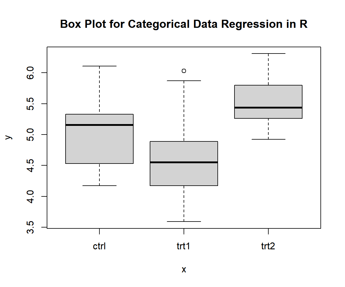
Box Plot for Categorical Data Regression in R
The appearance of the box plots suggests that there are differences in the group means and medians.
1.2 Run the Regression with the Categorical Independent Variable
Run the regression model with the categorical independent variable
using the lm() function, and print the results using the
summary() function.
group = PlantGrowth$group
weight = PlantGrowth$weight

# Regression with the categorical variable
model = lm(weight ~ group)
summary(model)
Or:
Call:
lm(formula = weight ~ group, data = PlantGrowth)

Residuals:
    Min      1Q  Median      3Q     Max
-1.0710 -0.4180 -0.0060  0.2627  1.3690

Coefficients:
            Estimate Std. Error t value Pr(>|t|)
(Intercept)   5.0320     0.1971  25.527   <2e-16 ***
grouptrt1    -0.3710     0.2788  -1.331   0.1944
grouptrt2     0.4940     0.2788   1.772   0.0877 .
---
Signif. codes:  0 '***' 0.001 '**' 0.01 '*' 0.05 '.' 0.1 ' ' 1

Residual standard error: 0.6234 on 27 degrees of freedom
Multiple R-squared:  0.2641,    Adjusted R-squared:  0.2096
F-statistic: 4.846 on 2 and 27 DF,  p-value: 0.01591
1.3 Interpretation of the Categorical Data Regression Results
- Effects (or coefficients):
- The estimated mean for the "ctrl" group is the intercept, \(\text{summary(model)\$coefficients[1, 1]}\)
\(= 5.032\).
This is because "ctrl" is the first group in the alphanumeric order. - The estimated mean for the "trt1" group is \(\text{the intercept + the effect of trt1 vs. ctrl}\), \(\text{summary(model)\$coefficients[1, 1]}\) \(+\) \(\text{summary(model)\$coefficients[2, 1]}\) \(= 5.032 + (-0.371)\) \(= 4.661\).
- The estimated mean for the "trt2" group is \(\text{the intercept + the effect of trt2 vs. ctrl}\), \(\text{summary(model)\$coefficients[1, 1]}\) \(+\) \(\text{summary(model)\$coefficients[3, 1]}\) \(= 5.032 + 0.494\) \(= 5.526\).
- The estimated mean for the "ctrl" group is the intercept, \(\text{summary(model)\$coefficients[1, 1]}\)
\(= 5.032\).
- P-values:
For level of significance, \(\alpha = 0.1\).- The p-value for the intercept which is also the p-value for the "ctrl" group, is \(\text{summary(model)\$coefficients[1, 4]} \approx 0\). Since the p-value is less than \(0.1\), we say that the mean of the "ctrl" group is significantly different from \(0\).
- The p-value for the "trt1" group is, \(\text{summary(model)\$coefficients[2, 4]}\) \(=0.194\). Since the p-value is greater than \(0.1\), we say that the effect (or mean) of the "trt1" group is NOT significantly different from that of the "ctrl" group.
- The p-value for the "trt2" group is, \(\text{summary(model)\$coefficients[3, 4]}\) \(=0.088\). Since the p-value is less than \(0.1\), we say that the effect (or mean) of the "trt2" group is significantly different from that of the "ctrl" group.
- R-squared:
The r-squared value is \(\text{summary(model)\$r.squared}\) \(=0.264\). This means that the model, using the treatments, explains \(26.4\%\) of the variation in the dependent variable \(y\) (weights) from the sample mean of \(y\), \(\bar y\).
1.4 Prediction and Estimation
To predict or estimate weights for any plant:
If the plant is from the "ctrl" group we can use the intercept, \(5.032\). This is because the "ctrl" group is represented as the intercept on the table.
If the plant is from the "trt1" group, we can use, \(5.032 + (-0.371)\) \(=4.661\).
If the plant is from the "trt2" group, we can use, \(5.032 + 0.494\) \(=5.526\).
 ctrl  trt1  trt2
5.032 4.661 5.526
2 Regression with Multiple Categorical Independent Variables in R
Using the "warpbreaks" data from the "datasets" package, with 10 sample rows from 54 rows below.
   breaks wool tension
1      26    A       L
10     18    A       M
11     21    A       M
18     36    A       M
25     28    A       H
31     19    B       L
38     26    B       M
39     19    B       M
45     29    B       M
54     28    B       H
NOTE: The dependent variable is "breaks", and the independent variables are "wool" and "tension".
Check for Distribution by the Combination of Levels in the Factors
Use a side-by-side box plot to visually check for the distribution by the combinations of levels in the factors, and the differences in the group medians.
wool = warpbreaks$wool
tension = warpbreaks$tension
breaks = warpbreaks$breaks
boxplot(breaks ~ wool + tension,
     main = "Box Plot for Multiple Categorical Data Regression in R")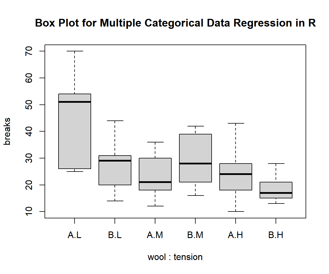
Box Plot for Multiple Categorical Data Regression in R
The appearance of the box plots suggests differences in the group medians and means.
2.1 Without Interaction Effect
Run the Regression
Run the regression model with the multiple categorical variables
using the lm() function, and print the results using the
summary() function.
wool = warpbreaks$wool
tension = warpbreaks$tension
breaks = warpbreaks$breaks

# Run the regression without interaction effect
model = lm(breaks ~ wool + tension)
summary(model)
Or:
# Run the regression without interaction effect
model = lm(breaks ~ wool + tension, data = warpbreaks)
summary(model)
Call:
lm(formula = breaks ~ wool + tension, data = warpbreaks)

Residuals:
    Min      1Q  Median      3Q     Max
-19.500  -8.083  -2.139   6.472  30.722

Coefficients:
            Estimate Std. Error t value Pr(>|t|)
(Intercept)   39.278      3.162  12.423  < 2e-16 ***
woolB         -5.778      3.162  -1.827 0.073614 .
tensionM     -10.000      3.872  -2.582 0.012787 *
tensionH     -14.722      3.872  -3.802 0.000391 ***
---
Signif. codes:  0 '***' 0.001 '**' 0.01 '*' 0.05 '.' 0.1 ' ' 1

Residual standard error: 11.62 on 50 degrees of freedom
Multiple R-squared:  0.2691,    Adjusted R-squared:  0.2253
F-statistic: 6.138 on 3 and 50 DF,  p-value: 0.00123
Interpretation: Multiple Categorical Variables Regression without Interaction
Note: A design where each level of one factor has the same number of observations for each level of the other factor.
Effects (or coefficients):
- Given that this is an orthogonal design without interaction effects,
the intercept is (4 \(\times\) overall
mean) \(-\) (mean of "woolB" \(+\) mean of "tensionM" \(+\) mean of "tensionH"), which is, \(\text{summary(model)\$coefficients[1, 1]}\)
\(= 39.278\).
Hence "woolA" and "tensionL" are the intercept given that they are the first levels in their factors in the alphanumeric order.
The calculation has \(4\) because there are \(3\) different effects in the table. - The effect of "woolB" versus "woolA" is, \(\text{summary(model)\$coefficients[2, 1]}\) \(= -5.778\). Given that this is an orthogonal design without interaction effects, this is the same as the (mean of "woolB" \(-\) mean of "woolA").
- The effect of "tensionM" versus "tensionL" is, \(\text{summary(model)\$coefficients[3, 1]}\) \(= -10\). Given that this is an orthogonal design without interaction effects, this is the same as the (mean of "tensionM" \(-\) mean of "tensionL").
- The effect of "tensionH" versus "tensionL" is, \(\text{summary(model)\$coefficients[4, 1]}\) \(= -14.722\). Given that this is an orthogonal design without interaction effects, this is the same as the (mean of "tensionH" \(-\) mean of "tensionL").
See below for illustrative calculations.
- Given that this is an orthogonal design without interaction effects,
the intercept is (4 \(\times\) overall
mean) \(-\) (mean of "woolB" \(+\) mean of "tensionM" \(+\) mean of "tensionH"), which is, \(\text{summary(model)\$coefficients[1, 1]}\)
\(= 39.278\).
P-values:
Difference in effects here also implies difference in means, as this is an orthogonal design.
For level of significance, \(\alpha = 0.05\).- The p-value for the intercept, or "woolA" and "tensionL" combination effect is, \(\text{summary(model)\$coefficients[1, 4]}\) \(\approx 0\). Since the p-value is less than \(0.05\), we say that the effect of the combination is significantly different from zero.
- The p-value for the effect of "woolB" versus "woolA" is, \(\text{summary(model)\$coefficients[2, 4]}\) \(= 0.074\). Since the p-value is greater than \(0.05\), we say that the effects of the two groups are NOT significantly different.
- The p-value for the effect of "tensionM" versus "tensionL" is, \(\text{summary(model)\$coefficients[3, 4]}\) \(=0.013\). Since the p-value is less than \(0.05\), we say that the effects of the two groups are significantly different.
- The p-value for the effect of "tensionH" versus "tensionL is, \(\text{summary(model)\$coefficients[4, 4]}\) \(=3.9\times 10^{-4}\). Since the p-value is less than \(0.05\), we say that the effects of the two groups are significantly different.
# For woolB
woolmeans = tapply(warpbreaks$breaks, warpbreaks$wool, mean)
woolmeans; woolmeans[2] - woolmeans[1]
A B
31.03704 25.25926 B
-5.777778 # For tensionM and tensionH
tensionmeans = tapply(warpbreaks$breaks, warpbreaks$tension, mean)
tensionmeans; tensionmeans[2:3] - tensionmeans[1] L M H
36.38889 26.38889 21.66667 M H
-10.00000 -14.72222 [1] 39.27777Prediction and Estimation
To predict or estimate breaks for any combination of levels from the factors:
For "woolA" and "tensionL" group, use the intercept, \(39.278\). This is because "WoolA" and "tensionL" group are represented by the intercept on the table.
For "woolA" and "tensionM" group, use, \(39.278 + (-10)\) \(=29.278\).
For "woolA" and "tensionH" group, use, \(39.278 + (-14.722)\) \(=24.556\).
For "woolB" and "tensionL" group, use, \(39.278 + (-5.778)\) \(=33.5\).
For "woolB" and "tensionM" group, use, \(39.278 + (-5.778) + (-10)\) \(=23.5\).
For "woolB" and "tensionH" group, use, \(39.278 + (-5.778) + (-14.722)\) \(=18.778\).
2.2 With Interaction Effects
Run the Regression
Run the regression model with the multiple categorical variables
including interaction effects using the lm() function, and
print the results using the summary() function.
wool = warpbreaks$wool
tension = warpbreaks$tension
breaks = warpbreaks$breaks

# Run the regression with interaction effects
model = lm(breaks ~ wool + tension + wool:tension)
summary(model)
Or:
# Run the regression with interaction effects
model = lm(breaks ~ wool + tension + wool:tension, data = warpbreaks)
summary(model)
Call:
lm(formula = breaks ~ wool + tension + wool:tension, data = warpbreaks)

Residuals:
     Min       1Q   Median       3Q      Max
-19.5556  -6.8889  -0.6667   7.1944  25.4444

Coefficients:
               Estimate Std. Error t value Pr(>|t|)
(Intercept)      44.556      3.647  12.218 2.43e-16 ***
woolB           -16.333      5.157  -3.167 0.002677 **
tensionM        -20.556      5.157  -3.986 0.000228 ***
tensionH        -20.000      5.157  -3.878 0.000320 ***
woolB:tensionM   21.111      7.294   2.895 0.005698 **
woolB:tensionH   10.556      7.294   1.447 0.154327
---
Signif. codes:  0 '***' 0.001 '**' 0.01 '*' 0.05 '.' 0.1 ' ' 1

Residual standard error: 10.94 on 48 degrees of freedom
Multiple R-squared:  0.3778,    Adjusted R-squared:  0.3129
F-statistic: 5.828 on 5 and 48 DF,  p-value: 0.0002772
Interpretation: Multiple Categorical Variables Regression with Interaction
- P-values:
For level of significance, \(\alpha = 0.05\).- The p-value for "woolB" being lower than \(0.05\) means that the level of "wool" is statistically significant.
- The p-value for "tensionM" and "tensionH" being lower than \(0.05\) means that the level of "tension" is statistically significant.
- The p-value for the interaction effect of "woolB:tensionM" being lower than \(0.05\) means that the combination or interaction of the levels of "wool" and "tension" is statistically significant.
- R-squared:
The r-squared value is \(\text{summary(model)\$r.squared}\) \(=0.378\). This means that the model, using the "wool" and "tension" factors, and their interaction effects, explains \(37.8\%\) of the variation in the dependent variable \(y\) (breaks) from the sample mean of \(y\), \(\bar y\).
Prediction and Estimation
To predict or estimate breaks for any combination of levels from the factors using the effects from the corresponding levels of the factors and the interaction effects:
For "woolA" and "tensionL" group, use the intercept, \(44.556\). This is because "woolA" and "tensionL" groups are represented by the intercept given that they are the first levels in their factors in the alphanumeric order, hence, they do not appear on the table.
For "woolA" and "tensionM" group, use, \(44.556 + (-20.556)\) \(=24\).
For "woolA" and "tensionH" group, use, \(44.556 + (-20)\) \(=24.556\).
For "woolB" and "tensionL" group, use, \(44.556 + (-16.333)\) \(=28.222\).
For "woolB" and "tensionM" group, use, \(44.556 + (-16.333) + (-20.556) + 21.111\) \(=28.778\).
For "woolB" and "tensionH" group, use, \(44.556 + (-16.333) + (-20) + 10.556\) \(=18.778\).
With the interaction effects included, the predictions or estimates are the same as the in-sample means for each combination of factor levels. See results below.
     A:L      A:M      A:H      B:L      B:M      B:H
44.55556 24.00000 24.55556 28.22222 28.77778 18.77778 The feedback form is a Google form but it does not collect any personal information.
Please click on the link below to go to the Google form.
Thank You!
Go to Feedback Form
Copyright © 2020 - 2026. All Rights Reserved by Stats Codes