1 Normal Distribution Test Based on Histogram in R

Here we test for normality using histograms, density histograms, and normal distribution density plots.

Sample 1

For example, for a sample of \(600\) observations from the normal distribution with \(\tt{mean = 12}\) and \(\tt{sd = 3}\), we can assess if it is from a normal distribution.

hs_sample = rnorm(600, 12, 3)

Plots 1

We can plot the histogram, and a density histogram overlaid with both the sample density and normal density. The more bell-shaped the histogram appears to be, the more likely the sample is from a normal distribution. Similarly, the more the sample density line and the normal distribution density line overlap, the more likely the sample is from a normal distribution.

Based on the appearances below, as expected, we can conclude the sample is from a normal distribution.

# Histogram Code
hist(hs_sample,
     main = "Histogram of Sample",
     xlab = "Observations",
     ylab = "Frequency",
     xlim = c(0, 24),
     ylim = c(0, 200))

# Density Histogram
hist(hs_sample, freq = FALSE,
     main = "Density Histogram of Sample",
     xlab = "Observations",
     ylab = "Density",
     xlim = c(0, 24),
     ylim = c(0, 0.2))

# Sample Density
den = density(hs_sample)
lines(den, col = "blue", lwd = 1.5)

# Normal Density
x = seq(0, 24, by = 1/1000)
y = dnorm(x, mean(hs_sample), sd(hs_sample))
points(x, y, type = 'l', col = "green", lwd = 2)
legend("topright", c("Sample", "Normal"),
       fill = c("blue", "green"))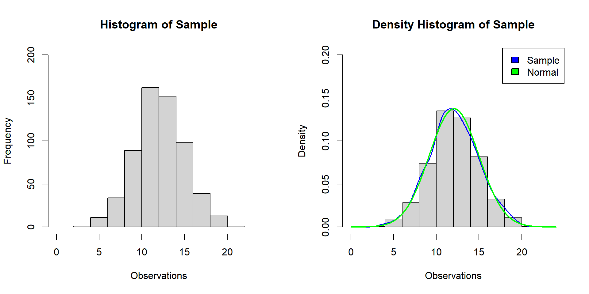

Example 1: Histogram and Density Histogram for Normality Test in R

Sample 2

For example, for a sample of \(600\) observations from the exponential distribution with \(\tt{rate = 1/12}\) or \(\tt{mean = 12}\), we can assess if it is from a normal distribution.

hs_sample2 = rexp(600, 1/12)

Plots 2

Based on the appearances below, as expected, we can conclude the sample is NOT from a normal distribution.

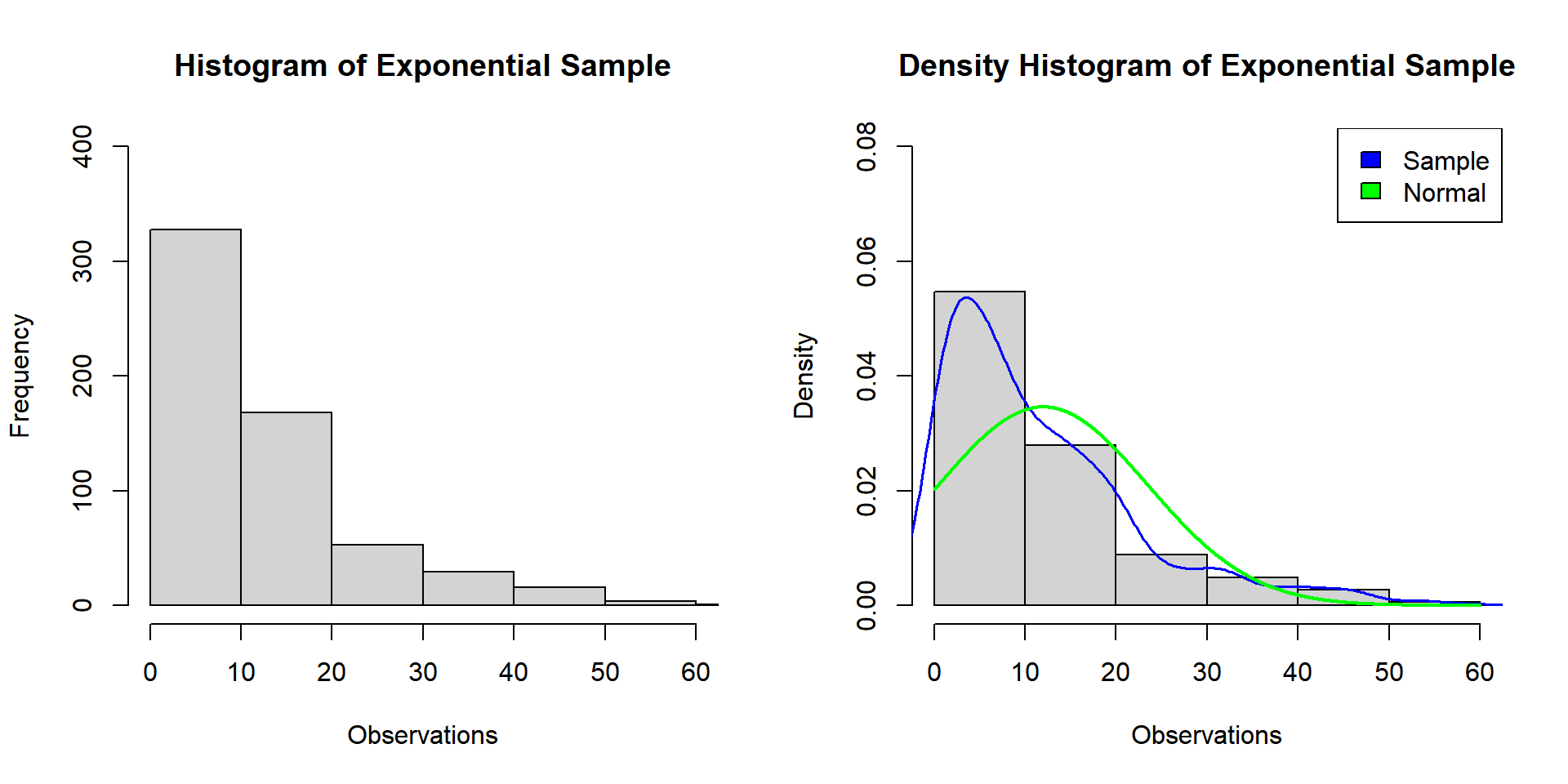
Example 2: Histogram and Density Histogram for Normality Test in R

2 Normal Distribution Test Based on Quantile-Quantile Plot in R

Here we test for normality using quantile-quantile plots.

Sample 1

For example, for a sample of \(200\) observations from the normal distribution with \(\tt{mean = 3}\) and \(\tt{sd = 1}\), we can assess if it is from a normal distribution.

qq_sample = rnorm(200, 3, 1)

Plots 1

In the Q-Q plot, the more the dots align to a straight line, the more likely the sample is from a normal distribution.

Based on the appearances below, as expected, we can conclude the sample is from a normal distribution.

# Simple Q-Q Plot Code
qqnorm(qq_sample)
       
# Q-Q Plot Code with Line Overlaid
qqnorm(qq_sample,
     main = "Sample Normal Q-Q Plot",
     xlab = "Quantiles from Normal Distribution",
     ylab = "Quantiles from Sample")
qqline(qq_sample, col = "red", lwd = "2")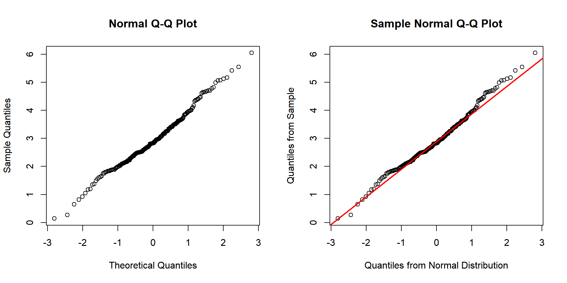

Example 1: Normal Q-Q Plot for Normality Test in R

Sample 2

For example, for a sample of \(100\) observations from the exponential distribution with \(\tt{rate = 1/3}\) or \(\tt{mean = 3}\), we can assess if it is from a normal distribution.

qq_sample2 = rexp(100, 1/3)

Plots 2

Based on the appearances below, as expected, we can conclude the sample is NOT from a normal distribution.

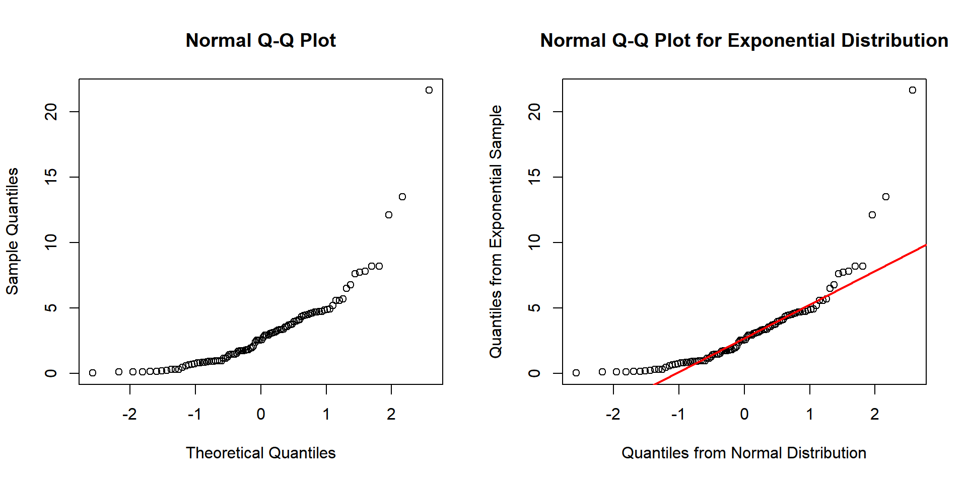
Example 2: Normal Q-Q Plot for Normality Test in R

3 Normal Distribution Test Based on Shapiro-Wilk Test in R

The normal distribution test null and alternate hypotheses are:

• \(H_0\): The sample is from a normal distribution.

• \(H_1\): The sample is NOT from a normal distribution.

The test-statistic is \(W\), the lower the value of \(W\), the more the distribution is likely to be different from a normal distribution, leading to a smaller p-value.

Example 1:

The sample of interest here is a sample of \(60\) observations from the normal distribution with \(\tt{mean = 4}\) and \(\tt{sd = 1.5}\).

sw_sample = rnorm(60, 4, 1.5)

With level of significance \(\alpha = 0.05\), test if the sample is from a normal distribution.

shapiro.test(sw_sample)

    Shapiro-Wilk normality test

data:  sw_sample
W = 0.99291, p-value = 0.98

As expected, we have high \(W\), and high \(\tt{p-value}\;(0.98)\) above the level of significance \((\alpha = 0.05)\). Hence, we fail to reject \(H_0\) that the sample is from a normal distribution.

Example 2:

The sample of interest here is a sample of \(100\) observations from the exponential distribution with \(\tt{rate = 1/4}\) or \(\tt{mean = 4}\).

sw_sample2 = rexp(100, 1/4)

With level of significance \(\alpha = 0.05\), test if the sample is from a normal distribution.

shapiro.test(sw_sample2)

    Shapiro-Wilk normality test

data:  sw_sample2
W = 0.76107, p-value = 1.856e-11

As expected, we have low \(W\), and low \(\tt{p-value}\;(1.856e-11)\) below the level of significance \((\alpha = 0.05)\). Hence, we reject \(H_0\) that the sample is from a normal distribution.

4 Normal Distribution Test Based on Kolmogorov-Smirnov Test in R

The one-sample normal distribution test null and alternate hypotheses are:

• \(H_0\): The sample is from the normal distribution with \(\tt{mean}\) and \(\tt{sd}\) specified.

• \(H_1\): The sample is NOT from the normal distribution.

The test-statistic is \(D\), the higher the value of \(D\), the more different the distribution is from a normal distribution, leading to a smaller p-value.

The sample of interest here is a sample of \(60\) observations from the normal distribution with \(\tt{mean = 8}\) and \(\tt{sd = 3}\).

ks_sample = rnorm(60, 8, 3)

Example 1:

With level of significance \(\alpha = 0.05\), test if the sample is from the normal distribution with \(\tt{mean = 8}\) and \(\tt{sd = 3}\).

ks.test(ks_sample, pnorm, 8, 3)

    Exact one-sample Kolmogorov-Smirnov test

data:  ks_sample
D = 0.083034, p-value = 0.7713
alternative hypothesis: two-sided

As expected, we have low \(D_n\), and high \(\tt{p-value}\;(0.7713)\) above the level of significance \((\alpha = 0.05)\). Hence, we fail to reject \(H_0\) that the sample is from \(X \sim N(8, 3)\).

Example 2:

With level of significance \(\alpha = 0.05\), test if the sample is from the normal distribution with \(\tt{mean = 5}\) and \(\tt{sd = 2}\).

ks.test(ks_sample, pnorm, 5, 2)

    Exact one-sample Kolmogorov-Smirnov test

data:  ks_sample
D = 0.53547, p-value = 6.661e-16
alternative hypothesis: two-sided

As expected, we have high \(D_n\), and low \(\tt{p-value}\;(6.661e-16)\) below the level of significance \((\alpha = 0.05)\). Hence, we reject \(H_0\) that the sample is from \(X \sim N(5, 2)\).