One Proportion Tests (with Z & Chi-squared) in R
- 1 Test Statistic for One Proportion Test in R
- 2 Simple One Proportion Test in R
- 3 One Proportion Test Critical Value in R
- 4 Two-tailed One Proportion Test in R
- 5 One-tailed One Proportion Test in R
- 6 One Proportion Test: Test Statistics, P-value & Degree of Freedom in R
- 7 One Proportion Test: Estimate & Confidence Interval in R
Here, we discuss the one proportion tests in R with interpretations, including, chi-squared values, p-values, critical values, and confidence intervals.
The one proportion test in R can be performed with the
prop.test() function from the base "stats" package.
The one proportion test can be used to test whether the proportion of successes in the population where an independent random sample comes from is equal to a certain value (which is stated in the null hypothesis) or not.
In the one proportion test, the test statistic follows a chi-squared distribution with 1 degree of freedom (or standard normal distribution) when the null hypothesis is true.
| Question | Is the proportion equal to \(p_0\)? | Is the proportion greater than \(p_0\)? | Is the proportion less than \(p_0\)? |
| Form of Test | Two-tailed | Right-tailed test | Left-tailed test |
| Null Hypothesis, \(H_0\) | \(p = p_0\) | \(p = p_0\) | \(p = p_0\) |
| Alternate Hypothesis, \(H_1\) | \(p \neq p_0\) | \(p > p_0\) | \(p < p_0\) |
Sample Steps to Run a One Proportion Test:
# Specify:
# x as the number of successes
# n as the number of trials

# Run the one proportion test with specifications

prop.test(x = 60, n = 100, p = 0.5,
          alternative = "two.sided",
          conf.level = 0.95,
          correct = FALSE)
    1-sample proportions test without continuity correction

data:  60 out of 100, null probability 0.5
X-squared = 4, df = 1, p-value = 0.0455
alternative hypothesis: true p is not equal to 0.5
95 percent confidence interval:
 0.5020026 0.6905987
sample estimates:
  p
0.6 | Argument | Usage |
| x | Sample count of number of successes |
| n | Sample count of number of trials |
| p | Population proportion value in null hypothesis |
| alternative | Set alternate hypothesis as "greater", "less", or the default "two.sided" |
| conf.level | Level of confidence for the test and confidence interval (default = 0.95) |
| correct | Set to FALSE to remove continuity correction (default =
TRUE) |
Creating a One Proportion Test Object:
# Create object with:
# x as the number of successes
# n as the number of trials
prop_object = prop.test(x = 60, n = 100, p = 0.5,
                        alternative = "two.sided",
                        conf.level = 0.95,
                        correct = FALSE)

# Extract a component
prop_object$statistic
X-squared
4 | Test Component | Usage |
| prop_object$statistic | Test-statistic value |
| prop_object$p.value | P-value |
| prop_object$parameter | Degrees of freedom |
| prop_object$estimate | Point estimate or sample proportion |
| prop_object$conf.int | Confidence interval |
1 Test Statistic for One Proportion Test in R
For \(\chi^2_1\), which is the
chi-squared distribution with 1 degree of freedom, and \(z\), which is the standard normal
distribution (mean is 0, and standard
deviation is 1), the one proportion test has test statistics, \(\chi^2_1\) (or \(z^2\)), without continuity correction
(correct = FALSE), which takes the form:
\[z = \frac{\frac{x}{n} - p_0}{\sqrt \frac{p_0(1-p_0)}{n}} \quad \text{or} \quad \chi^2_1=\sum_{i=1}^{2}\frac{(O_i-E_i)^2}{E_i}.\]
In cases where Yates’ continuity correction is applied (default in R), it takes the form:
\[z = \frac{\frac{(x \pm c)}{n} - p_0}{\sqrt \frac{p_0(1-p_0)}{n}} \quad \text{or} \quad \chi^2_1=\sum_{i=1}^{2}\frac{(|O_i-E_i|-c)^2}{E_i}.\] Note that \(z^2 = \chi^2_1\) in both cases. However, for one-sided tests, the level of significance \(\alpha\) for \(z\) is \(2\alpha\) for \(\chi^2_1\).
| \(z\) test | \(\chi^2_1\) test |
|---|---|
| \(x\) is the number of successes, \(n\) is the number of trials | \(O_i's\) are the observed values (\(O_1 = x\), and \(O_2 = n-x\)) |
| \(p_0\) is the population proportion value to be tested and set in the null hypothesis | \(E_i's\) are the expected values (\(E_1 = np_0\), and \(E_2 = n(1-p_0)\)) |
|
\(c = \min\{0.5, |np_0-x|\}\): \(x+c\) when \(np_0 \geq x\), and \(x-c\) when \(np_0 < x\) |
\(c = \min\{0.5, |np_0-x|\}\) |
The test is ideal for large samples sizes (for example, \(np_0 > 5\) \(\&\) \(n(1-p_0) > 5\)).
See the exact binomial test for exact p-values. See also the two proportions test.
2 Simple One Proportion Test in R
With number of successes, \(x = 55\) in \(n = 100\) trials.
For the following null hypothesis \(H_0\), and alternative hypothesis \(H_1\), with the level of significance \(\alpha=0.05\), applying continuity correction.
\(H_0:\) the population proportion is equal to 0.5 (\(p = 0.5\)).
\(H_1:\) the population proportion is not equal to 0.5 (\(p \neq 0.5\), hence the default two-sided).
Because the level of significance is \(\alpha=0.05\), the level of confidence is \(1 - \alpha = 0.95\).
The prop.test() function has the default
proportion as 0.5, the default alternative as
"two.sided", the default level of confidence as
0.95, and the default method as continuity
corrected, hence, you do not need to specify the "p",
"alternative", "conf.level" and "correct" arguments in this
case.
Or:
    1-sample proportions test with continuity correction

data:  55 out of 100, null probability 0.5
X-squared = 0.81, df = 1, p-value = 0.3681
alternative hypothesis: true p is not equal to 0.5
95 percent confidence interval:
 0.4475426 0.6485719
sample estimates:
   p
0.55
The sample proportion, \(\hat p = x/n\), is 0.55,
test statistic, \(\chi^2_1\), is 0.81,
the degree of freedom is 1,
the p-value, \(p\), is 0.3681,
the 95% confidence interval is [0.4475426, 0.6485719].
Interpretation:
Note that for prop.test() in R, the one proportion
test’s p-value and T-statistic methods may disagree with the confidence
interval method for some edge cases. This is because the p-value and
T-statistic are based on the chi-squared (or equivalent standard normal)
distribution, while the confidence interval is based on the Wilson
Score method.
P-value: With the p-value (\(p = 0.3681\)) being greater than the level of significance 0.05, we fail to reject the null hypothesis that the population proportion is equal to 0.5.
\(\chi^2_1\) T-statistic: With test statistics value (\(\chi^2_1 = 0.81\)) being less than the critical value, \(\chi^2_{1,\alpha}=\text{qchisq(0.95, 1)}=3.8414588\) (or not in the shaded region), we fail to reject the null hypothesis that the population proportion is equal to 0.5.
\(z\) T-statistic: With test statistics value (\(z=0.9=\sqrt{\chi^2_1 = 0.81}\)) being between than the critical values, \(-z_{\alpha/2}=\text{qnorm(0.025)}=-1.959964\) \(=-\sqrt{\text{qchisq(0.95, 1)}=3.8414588}\) and \(z_{\alpha/2}=\text{qnorm(0.975)}=1.959964\) \(=\sqrt{\text{qchisq(0.95, 1)}=3.8414588}\) (or not in the shaded region), we fail to reject the null hypothesis that the population proportion is equal to 0.5.
Confidence Interval: With the null hypothesis proportion value (\(p = 0.5\)) being inside the confidence interval, \([0.4475426, 0.6485719]\), we fail to reject the null hypothesis that the population proportion is equal to 0.5.
par(mfrow=c(1,2))
#Plot Chi-squared
x = seq(0.01, 8, 1/1000); y = dchisq(x, df=1)
plot(x, y, type = "l",
     xlim = c(0, 8), ylim = c(-0.1, min(max(y), 1)),
     main = "One Proportion Test
Shaded Region for Simple Test",
     xlab = "x", ylab = "Density",
     lwd = 2, col = "blue")
abline(h=0)
# Add shaded region and legend
point = qchisq(0.95, 1)
polygon(x = c(x[x >= point], 8, point),
        y = c(y[x >= point], 0, 0),
        col = "blue")
legend("topright", c("Area = 0.05"),
       fill = c("blue"), inset = 0.01)
# Add critical value and chi-value
arrows(2, 0.4, 0.81, 0)
text(2, 0.45, "chi-squared = 0.81")
text(3.841459, -0.06, expression(chi[1][','][alpha]^2==3.841459))
#Plot z
x = seq(-4, 4, 1/1000); y = dnorm(x)
plot(x, y, type = "l",
     xlim = c(-4, 4), ylim = c(-0.03, max(y)),
     main = "One Proportion Test
Shaded Region for Simple Test",
     xlab = "x", ylab = "Density",
     lwd = 2, col = "blue")
abline(h=0)
# Add shaded region and legend
point1 = qnorm(0.025); point2 = qnorm(0.975)
polygon(x = c(-4, x[x <= point1], point1),
        y = c(0, y[x <= point1], 0),
        col = "blue")
polygon(x = c(x[x >= point2], 4, point2),
        y = c(y[x >= point2], 0, 0),
        col = "blue")
legend("topright", c("Area = 0.05"),
       fill = c("blue"), inset = 0.01)
# Add critical value and z-value
arrows(0, 0.1, 0.9, 0)
text(0, 0.12, expression(z==0.9))
text(-1.959964, -0.02, expression(-z[alpha/2]==-1.959964))
text(1.959964, -0.02, expression(z[alpha/2]==1.959964))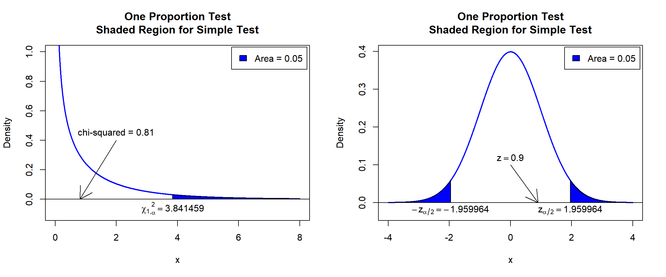
One Proportion Test Shaded Region for Simple Test in R
See line charts, shading areas under a curve, lines & arrows on plots, mathematical expressions on plots, and legends on plots for more details on making the plots above.
3 One Proportion Test Critical Value in R
To get the critical value for a one proportion test in R, you can use
the qchisq() function for chi-squared distribution, or the
qnorm() function for the standard normal distribution to
derive the quantile associated with the given level of significance
value \(\alpha\).
For two-tailed test with level of significance \(\alpha\). The critical values are: for chi-squared, qchisq(\(1-\alpha\), 1), or for \(z\), qnorm(\(\alpha/2\)) and qnorm(\(1-\alpha/2\)).
For one-tailed test with level of significance \(\alpha\). The critical value is: for chi-squared, qchisq(\(1-2\alpha\), 1); or for \(z\), left-tailed, qnorm(\(\alpha\)), and for right-tailed, qnorm(\(1-\alpha\)).
Example:
For \(\alpha = 0.05\).
Two-tailed:
[1] 3.841459[1] -1.959964[1] 1.959964One-tailed:
[1] 2.705543[1] -1.644854[1] 1.6448544 Two-tailed One Proportion Test in R
With number of successes, \(x = 31\) in \(n = 100\) trials.
For the following null hypothesis \(H_0\), and alternative hypothesis \(H_1\), with the level of significance \(\alpha=0.1\), without continuity correction.
\(H_0:\) the population proportion is equal to 0.4 (\(p = 0.4\)).
\(H_1:\) the population proportion is not equal to 0.4 (\(p \neq 0.4\), hence the default two-sided).
Because the level of significance is \(\alpha=0.1\), the level of confidence is \(1 - \alpha = 0.9\).
    1-sample proportions test without continuity correction

data:  31 out of 100, null probability 0.4
X-squared = 3.375, df = 1, p-value = 0.06619
alternative hypothesis: true p is not equal to 0.4
90 percent confidence interval:
 0.2397737 0.3902365
sample estimates:
   p
0.31
Interpretation:
P-value: With the p-value (\(p = 0.06619\)) being lower than the level of significance 0.1, we reject the null hypothesis that the population proportion is equal to 0.4.
\(\chi^2_1\) T-statistic: With test statistics value (\(\chi^2_1 = 3.375\)) being in the critical region (shaded area), that is, \(\chi^2_1 = 3.375\) greater than \(\chi^2_{1, \alpha}=\text{qchisq(0.9, 1)}=2.7055435\), we reject the null hypothesis that the population proportion is equal to 0.4.
\(z\) T-statistic: With test statistics value (\(z=-1.8371173=-\sqrt{\chi^2_1 = 3.375}\)) being in the critical region (shaded area), that is, \(z=-1.8371173\) less than \(-z_{\alpha/2}=\text{qnorm(0.05)}=-1.6448536\) \(=-\sqrt{\text{qchisq(0.9, 1)}=2.7055435}\), we reject the null hypothesis that the population proportion is equal to 0.4.
Confidence Interval: With the null hypothesis proportion value (\(p = 0.4\)) being outside the confidence interval, \([0.2397737, 0.3902365]\), we reject the null hypothesis that the population proportion is equal to 0.4.
par(mfrow=c(1,2))
#Plot Chi-squared
x = seq(0.01, 8, 1/1000); y = dchisq(x, df=1)
plot(x, y, type = "l",
     xlim = c(0, 8), ylim = c(-0.1, min(max(y), 1)),
     main = "One Proportion Test
Shaded Region for Two-tailed Test",
     xlab = "x", ylab = "Density",
     lwd = 2, col = "blue")
abline(h=0)
# Add shaded region and legend
point = qchisq(0.9, 1)
polygon(x = c(x[x >= point], 8, point),
        y = c(y[x >= point], 0, 0),
        col = "blue")
legend("topright", c("Area = 0.1"),
       fill = c("blue"), inset = 0.01)
# Add critical value and chi-value
arrows(3.375, 0.4, 3.375, 0)
text(3.375, 0.45, "chi-squared = 3.375")
text(2.705543, -0.06, expression(chi[1][','][alpha]^2==2.705543))
#Plot z
x = seq(-4, 4, 1/1000); y = dnorm(x)
plot(x, y, type = "l",
     xlim = c(-4, 4), ylim = c(-0.03, max(y)),
     main = "One Proportion Test
Shaded Region for Two-tailed Test",
     xlab = "x", ylab = "Density",
     lwd = 2, col = "blue")
abline(h=0)
# Add shaded region and legend
point1 = qnorm(0.05); point2 = qnorm(0.95)
polygon(x = c(-4, x[x <= point1], point1),
        y = c(0, y[x <= point1], 0),
        col = "blue")
polygon(x = c(x[x >= point2], 4, point2),
        y = c(y[x >= point2], 0, 0),
        col = "blue")
legend("topright", c("Area = 0.1"),
       fill = c("blue"), inset = 0.01)
# Add critical value and z-value
arrows(0, 0.15, -1.837117, 0)
text(0, 0.17, expression(z==-1.837117))
text(-1.644854, -0.02, expression(-z[alpha/2]==-1.644854))
text(1.644854, -0.02, expression(z[alpha/2]==1.644854))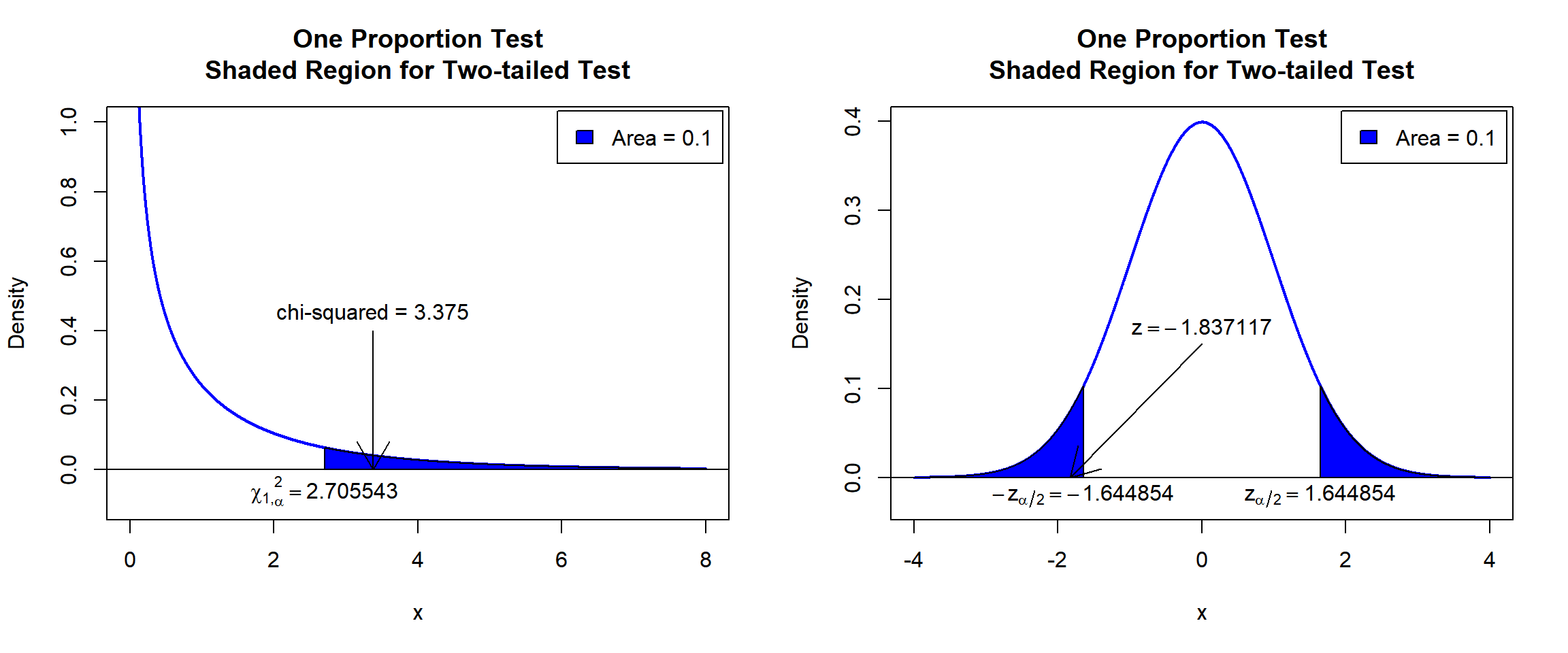
One Proportion Test Shaded Region for Two-tailed Test in R
5 One-tailed One Proportion Test in R
Right Tailed Test
With number of successes, \(x = 92\) in \(n = 120\) trials.
For the following null hypothesis \(H_0\), and alternative hypothesis \(H_1\), with the level of significance \(\alpha=0.1\), applying continuity correction.
\(H_0:\) the population proportion is equal to 0.65 (\(p = 0.65\)).
\(H_1:\) the population proportion is greater than 0.65 (\(p > 0.65\), hence one-sided).
Because the level of significance is \(\alpha=0.1\), the level of confidence is \(1 - \alpha = 0.9\).
    1-sample proportions test with continuity correction

data:  92 out of 120, null probability 0.65
X-squared = 6.6758, df = 1, p-value = 0.004886
alternative hypothesis: true p is greater than 0.65
90 percent confidence interval:
 0.7093813 1.0000000
sample estimates:
        p
0.7666667
Interpretation:
P-value: With the p-value (\(p = 0.004886\)) being less than the level of significance 0.1, we reject the null hypothesis that the population proportion is equal to 0.65.
\(\chi^2_1\) T-statistic: With test statistics value (\(\chi^2_1 = 6.6758\)) being in the critical region (shaded area), that is, \(\chi^2_1 = 6.6758\) greater than \(\chi^2_{1,2\alpha}=\text{qchisq(0.8, 1)}=1.6423744\), we reject the null hypothesis that the population proportion is equal to 0.65.
\(z\) T-statistic: With test statistics value (\(z=2.583757=\sqrt{\chi^2_1 = 6.6758}\)) being in the critical region (shaded area), that is, \(z=2.583757\) greater than \(z_{\alpha}=\text{qnorm(0.9)}=1.2815516\) \(=\sqrt{\text{qchisq(0.8, 1)}=1.6423744}\), we reject the null hypothesis that the population proportion is equal to 0.65.
Confidence Interval: With the null hypothesis proportion value (\(p = 0.65\)) being outside the confidence interval, \([0.7093813, 1.0)\), we reject the null hypothesis that the population proportion is equal to 0.65.
par(mfrow=c(1,2))
#Plot Chi-squared
x = seq(0.01, 8, 1/1000); y = dchisq(x, df=1)
plot(x, y, type = "l",
     xlim = c(0, 8), ylim = c(-0.1, min(max(y), 1)),
     main = "One Proportion Test
Shaded Region for Right-tailed Test",
     xlab = "x", ylab = "Density",
     lwd = 2, col = "blue")
abline(h=0)
# Add shaded region and legend
point = qchisq(0.8, 1)
polygon(x = c(x[x >= point], 8, point),
        y = c(y[x >= point], 0, 0),
        col = "blue")
legend("topright", c("Area = 0.2"),
       fill = c("blue"), inset = 0.01)
# Add critical value and chi-value
arrows(6.6758, 0.4, 6.6758, 0)
text(6.6758, 0.45, "chi-squared = 6.6758")
text(1.642374, -0.06, expression(chi[1][','][2*alpha]^2==1.642374))
#Plot z
x = seq(-4, 4, 1/1000); y = dnorm(x)
plot(x, y, type = "l",
     xlim = c(-4, 4), ylim = c(-0.03, max(y)),
     main = "One Proportion Test
Shaded Region for Right-tailed Test",
     xlab = "x", ylab = "Density",
     lwd = 2, col = "blue")
abline(h=0)
# Add shaded region and legend
point = qnorm(0.9)
polygon(x = c(x[x >= point], 4, point),
        y = c(y[x >= point], 0, 0),
        col = "blue")
legend("topright", c("Area = 0.1"),
       fill = c("blue"), inset = 0.01)
# Add critical value and z-value
arrows(2.583757, 0.15, 2.583757, 0)
text(2.583757, 0.17, expression(z==2.583757))
text(1.281552, -0.02, expression(z[alpha]==1.281552))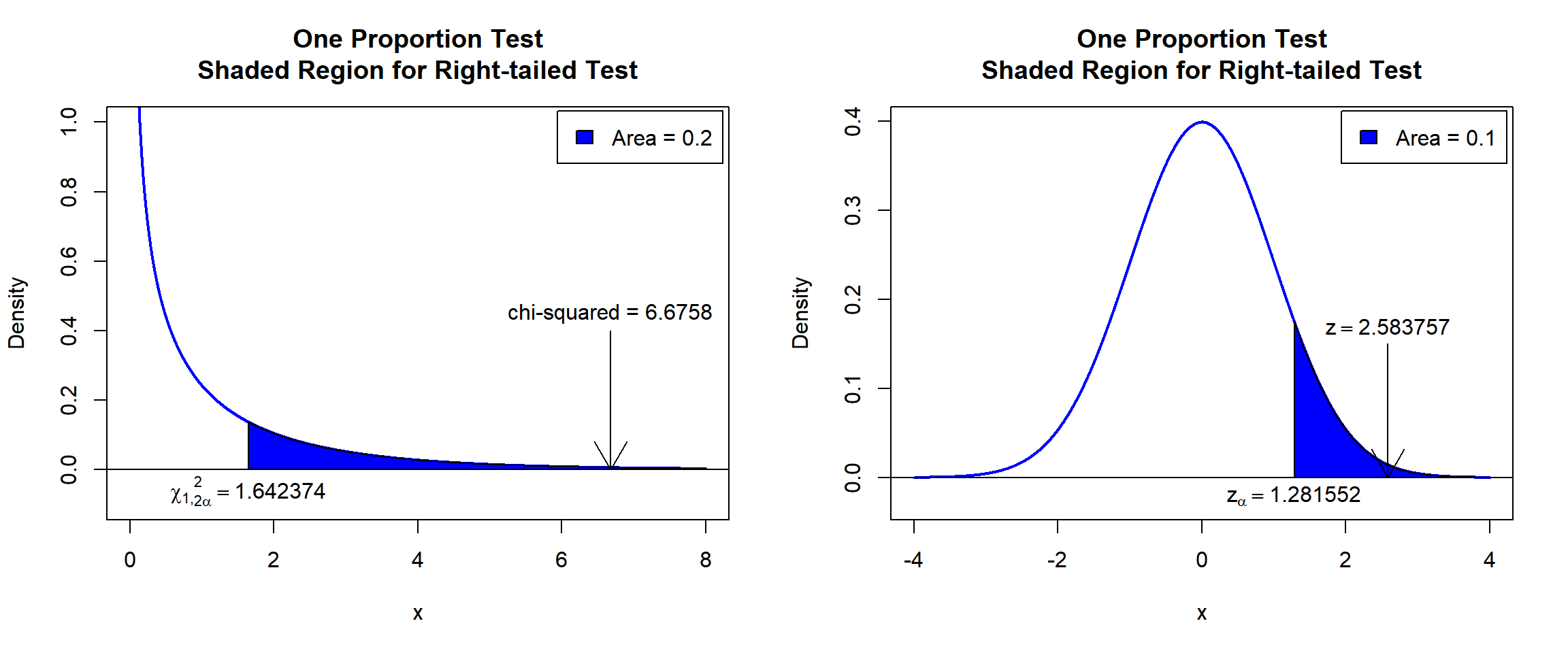
One Proportion Test Shaded Region for Right-tailed Test in R
Left Tailed Test
With number of successes, \(x = 24\) in \(n = 80\) trials.
For the following null hypothesis \(H_0\), and alternative hypothesis \(H_1\), with the level of significance \(\alpha=0.05\), without continuity correction.
\(H_0:\) the population proportion is equal to 0.35 (\(p=0.35\)).
\(H_1:\) the population proportion is less than 0.35 (\(p < 0.35\), hence one-sided).
Because the level of significance is \(\alpha=0.05\), the level of confidence is \(1 - \alpha = 0.95\).
    1-sample proportions test without continuity correction

data:  24 out of 80, null probability 0.35
X-squared = 0.87912, df = 1, p-value = 0.1742
alternative hypothesis: true p is less than 0.35
95 percent confidence interval:
 0.0000000 0.3896842
sample estimates:
  p
0.3
Interpretation:
P-value: With the p-value (\(p = 0.1742\)) being greater than the level of significance 0.05, we fail to reject the null hypothesis that the population proportion is equal to 0.35.
\(\chi^2_1\) T-statistic: With test statistics value (\(\chi^2_1 = 0.87912\)) being less than the critical value, \(\chi^2_{1,2\alpha}=\text{qchisq(0.9, 1)}=2.7055435\) (or not in the shaded region), we fail to reject the null hypothesis that the population proportion is equal to 0.35.
\(z\) T-statistic: With test statistics value (\(z=-0.937614=-\sqrt{\chi^2_1 = 0.87912}\)) being greater than the critical value, \(-z_{\alpha}=\text{qnorm(0.05)}=-1.6448536\) \(=-\sqrt{\text{qchisq(0.9, 1)}=2.7055435}\) (or not in the shaded region), we fail to reject the null hypothesis that the population proportion is equal to 0.35.
Confidence Interval: With the null hypothesis proportion value (\(p = 0.35\)) being inside the confidence interval, \((0, 0.3896842]\), we fail reject the null hypothesis that the population proportion is equal to 0.35.
par(mfrow=c(1,2))
#Plot Chi-squared
x = seq(0.01, 8, 1/1000); y = dchisq(x, df=1)
plot(x, y, type = "l",
     xlim = c(0, 8), ylim = c(-0.1, min(max(y), 1)),
     main = "One Proportion Test
Shaded Region for Left-tailed Test",
     xlab = "x", ylab = "Density",
     lwd = 2, col = "blue")
abline(h=0)
# Add shaded region and legend
point = qchisq(0.9, 1)
polygon(x = c(x[x >= point], 8, point),
        y = c(y[x >= point], 0, 0),
        col = "blue")
legend("topright", c("Area = 0.1"),
       fill = c("blue"), inset = 0.01)
# Add critical value and chi-value
arrows(2.5, 0.4, 0.87912, 0)
text(2.5, 0.45, "chi-squared = 0.87912")
text(2.705543, -0.06, expression(chi[1][','][2*alpha]^2==2.705543))
#Plot z
x = seq(-4, 4, 1/1000); y = dnorm(x)
plot(x, y, type = "l",
     xlim = c(-4, 4), ylim = c(-0.03, max(y)),
     main = "One Proportion Test
Shaded Region for Left-tailed Test",
     xlab = "x", ylab = "Density",
     lwd = 2, col = "blue")
abline(h=0)
# Add shaded region and legend
point = qnorm(0.05)
polygon(x = c(-4, x[x <= point], point),
        y = c(0, y[x <= point], 0),
        col = "blue")
legend("topright", c("Area = 0.05"),
       fill = c("blue"), inset = 0.01)
# Add critical value and z-value
arrows(0, 0.15, -0.937614, 0)
text(0, 0.17, expression(z==-0.937614))
text(-1.644854, -0.02, expression(-z[alpha]==-1.644854))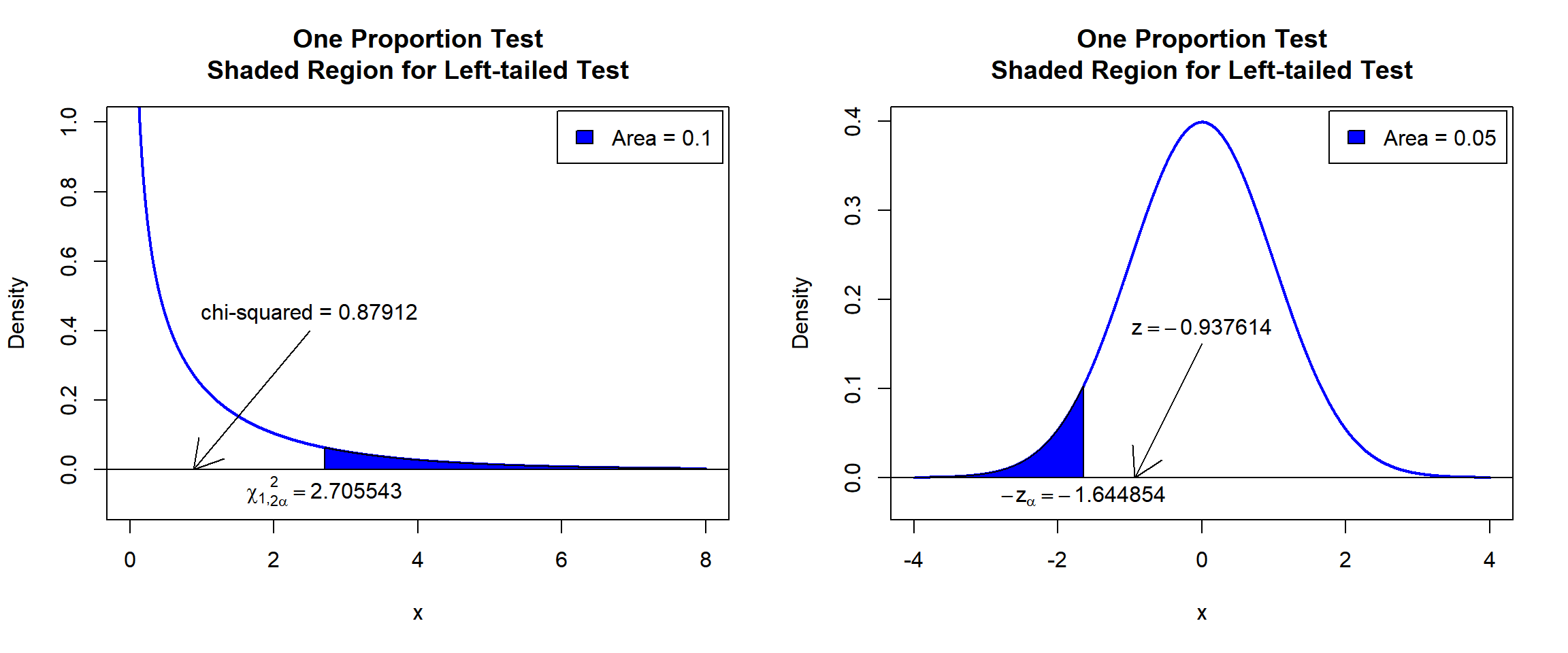
One Proportion Test Shaded Region for Left-tailed Test in R
6 One Proportion Test: Test Statistics, P-value & Degree of Freedom in R
Here for a one proportion test, we show how to get the test
statistics (or chi-squared value), p-values, and degrees of freedom from
the prop.test() function in R, or by written code.
x = 40; n = 65
prop_object = prop.test(x, n, p = 0.55,
                        alternative = "two.sided",
                        conf.level = 0.95,
                        correct = TRUE)
prop_object
    1-sample proportions test with continuity correction

data:  x out of n, null probability 0.55
X-squared = 0.87413, df = 1, p-value = 0.3498
alternative hypothesis: true p is not equal to 0.55
95 percent confidence interval:
 0.4861869 0.7308924
sample estimates:
        p
0.6153846
To get the test statistic or chi-squared value:
\[z = \frac{\frac{x}{n} - p_0}{\sqrt \frac{p_0(1-p_0)}{n}} \quad \text{or} \quad \chi^2_1=\sum_{i=1}^{2}\frac{(O_i-E_i)^2}{E_i}.\]
Applying Yates’ continuity correction, it takes the form:
\[z = \frac{\frac{(x \pm c)}{n} - p_0}{\sqrt \frac{p_0(1-p_0)}{n}} \quad \text{or} \quad \chi^2_1=\sum_{i=1}^{2}\frac{(|O_i-E_i|-c)^2}{E_i}.\]
\(c = \min\{0.5, |np_0-x|\}\), for \(z\) test statistic, \(x+c\) when \(np_0 \geq x\), and \(x-c\) when \(np_0<x\).
X-squared
0.8741259 [1] 0.8741259Same as (with continuity correction):
x = 40; n = 65; p = 0.55
c = min(0.5, abs(n*p-x))
cc = c*sign(n*p-x)
#z
z = ((x+cc)/n - p)/sqrt(p*(1-p)/n)
z
[1] 0.934947[1] 0.8741259[1] 0.8741259Without continuity correction:
#z
z = (x/n - p)/sqrt(p*(1-p)/n)
z
z^2 # convert to chi-squared
#chi-squared
chi = (abs(x-n*p)^2)/(n*p) + (abs((n-x)-n*(1-p))^2)/(n*(1-p))
chi
To get the p-value:
Two-tailed: With \(z = \sqrt{\chi^2_1}\): for positive test statistic (\(z^+\)), and negative test statistic (\(z^-\)).
For \(\chi^2_1\), \(P \left(\chi^2_1> \text{observed} \right)\).
For \(z\), \(Pvalue = 2*P(Z>z^+)\) or \(Pvalue = 2*P(Z<z^-)\).
One-tailed: For \(\chi^2_1\) is \(\frac{1}{2}*P \left(\chi^2_1> \text{observed} \right)\)
For \(z\), for right-tail, \(Pvalue = P(Z>z)\) or for left-tail, \(Pvalue = P(Z<z)\).
[1] 0.3498156Same as:
Note that the p-value depends on the \(\text{test statistics}\) (\(\chi^2_1 = 0.8741259\)), \(\text{degrees of freedom}\) (1), and \(z = \sqrt{\chi^2_1} = 0.934947\). We also
use the distribution functions pchisq() for the chi-squared
distribution and pnorm() for the standard normal
distribution in R.
[1] 0.3498156[1] 0.3498156[1] 0.3498156To get the degrees of freedom:
The degree of freedom is \(1\).
df
1 [1] 17 One Proportion Test: Estimate & Confidence Interval in R
Here for a one proportion test, we show how to get the sample
proportion and confidence interval from the prop.test()
function in R, or by written code.
x = 40; n = 60
prop_object = prop.test(x, n, p = 0.6,
                        alternative = "two.sided",
                        conf.level = 0.95,
                        correct = TRUE)
prop_object
    1-sample proportions test with continuity correction

data:  x out of n, null probability 0.6
X-squared = 0.85069, df = 1, p-value = 0.3564
alternative hypothesis: true p is not equal to 0.6
95 percent confidence interval:
 0.5320789 0.7798436
sample estimates:
        p
0.6666667
To get the point estimate or sample proportion:
\[\hat p = \frac{x}{n}.\]
        p
0.6666667 [1] 0.6666667Same as:
[1] 0.6666667To get the (Wilson Score) confidence interval for \(p\):
R uses the Wilson Score confidence interval.
With standard error estimate: \[\widehat{\text{SE}} = \sqrt {\frac {\hat p(1- \hat p)}{n}},\]
and \(c = 0.5\) with continuity correction, \(c=0\) without continuity correction.
For two-tailed:
With \(\hat p = \frac{x-c}{n}\), the lower bound is:
\[\left( \frac{n}{n + z_{\alpha/2}^2}\right)\left\{\left(\widehat{p} + \frac{z_{\alpha/2}^2}{2n}\right) - z_{\alpha/2}\sqrt{ \widehat{\text{SE}}^2 + \frac{z_{\alpha/2}^2}{4n^2}}\right\}.\] With \(\hat p = \frac{x+c}{n}\), the upper bound is:
\[\left( \frac{n}{n + z_{\alpha/2}^2}\right)\left\{\left(\widehat{p} + \frac{z_{\alpha/2}^2}{2n}\right) + z_{\alpha/2}\sqrt{ \widehat{\text{SE}}^2 + \frac{z_{\alpha/2}^2}{4n^2}}\right\}.\]
For right one-tailed with \(\hat p = \frac{x-c}{n}\), the interval is:
\[ \left[\left( \frac{n}{n + z_{\alpha}^2}\right)*\left\{\left(\widehat{p} + \frac{z_{\alpha}^2}{2n}\right) - z_{\alpha}\sqrt{ \widehat{\text{SE}}^2 + \frac{z_{\alpha}^2}{4n^2}}\right\} \;,\; 1 \right].\]
For left one-tailed with \(\hat p = \frac{x+c}{n}\), the interval is:
\[ \left[ 0 \;,\; \left\{\left(\widehat{p} + \frac{z_{\alpha}^2}{2n}\right) + z_{\alpha}\sqrt{ \widehat{\text{SE}}^2 + \frac{z_{\alpha}^2}{4n^2}} \right\}*\left( \frac{n}{n + z_{\alpha}^2}\right) \right].\]
[1] 0.5320789 0.7798436
attr(,"conf.level")
[1] 0.95[1] 0.5320789 0.7798436Same as:
x = 40; n = 60; alpha = 0.05
crit = qnorm(1-alpha/2)
# Continuity, set c = 0 for no continuity correction
c = 0.5
# Set scale
mult = (n/(n + crit^2))
# Lower
phat = (x-c)/n; SE = sqrt(phat*(1-phat)/n)
p_cent = phat + crit^2/(2*n)
margin = crit*sqrt(SE^2+crit^2/(4*n^2))
l = mult*(p_cent - margin)
# Upper
phat = (x+c)/n; SE = sqrt(phat*(1-phat)/n)
p_cent = phat + crit^2/(2*n)
margin = crit*sqrt(SE^2+crit^2/(4*n^2))
u = mult*(p_cent + margin)
# Bounds
c(l, u)
[1] 0.5320789 0.7798436One-tailed example:
x = 40; n = 60; alpha = 0.05
crit = qnorm(1-alpha)
# Continuity, set c = 0 for no continuity correction
c = 0.5
# Set scale
mult = (n/(n + crit^2))
# Right tail
phat = (x-c)/n; SE = sqrt(phat*(1-phat)/n)
p_cent = phat + crit^2/(2*n)
margin = crit*sqrt(SE^2+crit^2/(4*n^2))
l = mult*(p_cent - margin)
c(l, 1)
# Left tail
phat = (x+c)/n; SE = sqrt(phat*(1-phat)/n)
p_cent = phat + crit^2/(2*n)
margin = crit*sqrt(SE^2+crit^2/(4*n^2))
u = mult*(p_cent + margin)
c(0, u)
To get the simpler Wald confidence interval for \(p\):
For \(\hat p = \frac{x}{n}\), and standard error estimate, \(\widehat{\text{SE}} = \sqrt {\frac {\hat p(1- \hat p)}{n}}\).
For two-tailed:
\[CI = \left[\hat p - z_{\alpha/2}* \widehat{\text{SE}} \;,\; \hat p + z_{\alpha/2}* \widehat{\text{SE}} \right].\]
For right one-tailed:
\[CI = \left[\hat p - z_{\alpha}* \widehat{\text{SE}} \;,\; 1 \right].\]
For left one-tailed:
\[CI = \left[0 \;,\; \hat p + z_{\alpha}* \widehat{\text{SE}} \right].\]
x = 40; n = 60; alpha = 0.05; phat = x/n
SE = sqrt(phat*(1-phat)/n)
l = phat - qnorm(1-alpha/2)*SE
u = phat + qnorm(1-alpha/2)*SE
c(l, u)
[1] 0.5473871 0.7859463One-tailed example:
The feedback form is a Google form but it does not collect any personal information.
Please click on the link below to go to the Google form.
Thank You!
Go to Feedback Form
Copyright © 2020 - 2026. All Rights Reserved by Stats Codes