1 Test Statistic for One-way ANOVA Test in R
2 Simple One-way ANOVA Test in R
3 One-way ANOVA Test Critical Value in R
4 One-way ANOVA Test in R
5 One-way ANOVA Test: Test Statistics, P-value & Degrees of Freedom in R

Here, we discuss the one-way analysis of variance (ANOVA) test in R with interpretations, including, f-value, sum of squares, mean squares, p-values, and critical values.

The one-way ANOVA test in R can be performed with the anova() or oneway.test() function from the base "stats" package.

The one-way ANOVA test can be used to test whether the means of the populations where two or more independent random samples come from are equal (as stated in the null hypothesis) or not. With the typical equal variance assumption, it is an extension of the pooled two sample t-test from two means (or groups) to three or more means.

In the one-way ANOVA test, the test statistic follows an F-distribution when the null hypothesis is true.

One-way ANOVA Tests & Hypotheses
Question	Are the group means equal?
Null Hypothesis, $H_0$	$\mu_1 = \mu_2 = \dots = \mu_G$
Alternate Hypothesis, $H_1$	At least one group’s mean is different from the rest.

Sample Steps to Run a One-way ANOVA Test:

# Create the group data for the one-way ANOVA test
# Each row contains values for one group

y = c(7.2, 5.4, 5.2, 1.4,
      8.4, 4.8, 6.5,
      5.8, 6.2, 8.4, 4.8, 6.5)
groups = c("A", "A", "A", "A",
           "B", "B", "B",
           "C", "C", "C", "C", "C")

# Run the one-way ANOVA test with specifications

anova(lm(y ~ groups))

Analysis of Variance Table

Response: y
          Df Sum Sq Mean Sq F value Pr(>F)
groups     2  7.138  3.5690  1.0269 0.3965
Residuals  9 31.279  3.4754

# or
oneway.test(y ~ groups, var.equal = TRUE)


    One-way analysis of means

data:  y and groups
F = 1.0269, num df = 2, denom df = 9, p-value = 0.3965

Table of Some One-way ANOVA Tests Arguments in R
Argument (`anova()`)	Argument (`oneway.test()`)	Usage
lm(y ~ x)	y ~ x	y contains the sample data values, x specifies the group they belong.
	var.equal	Set to `TRUE` for equivalence with `anova()`. `FALSE` is unequal variance assumption, an extension of Welch’s t-test.

Creating a One-way ANOVA Test Object:

# Create data
y = rnorm(30)
groups = rep(c("A", "B", "C"), each = 10)

# Create object
aov_object = anova(lm(y ~ groups))
# or
owt_object = oneway.test(y~groups, var.equal = TRUE)

# Extract a component
aov_object$`F value`[1]

[1] 1.17051

# or
owt_object$statistic

      F 
1.17051

Table of Some One-way ANOVA Test Object Outputs in R
`anova()` Component	`oneway.test()` Component	Usage
aov_object$`F value`[1]	owt_object$statistic	Test-statistic value
aov_object$`Pr(>F)`[1]	owt_object$p.value	P-value
aov_object$Df	owt_object$parameter	Degrees of freedom
aov_object$`Sum Sq`		Sum of squares
aov_object$`Mean Sq`		Mean squares

1 Test Statistic for One-way ANOVA Test in R

The one-way analysis of variance test has test statistics, $F$, of the form:

\[\begin{align*} F & = \frac{\tt{variance \; between \; groups}}{\tt{variance \; within \; groups}} = \frac{MS_{groups}}{MS_{residuals}} \\ & = \frac{\left[ \sum_{j=1}^G N_j(\bar y_{j\cdot}-\bar y_{\cdot \cdot})^2 \right] / (G-1)}{\left[ \sum_{j=1}^G \sum_{k=1}^{N_j} (y_{jk}-\bar y_{j\cdot})^2 \right]/ (N-G)}\\ & = \frac{\left[ \sum_{j=1}^G N_j(\bar y_{j.}-\bar y_{\cdot \cdot})^2 \right]/ (G-1)}{\left[ \sum_{j=1}^G (N_j-1) s_j^2 \right]/ (N-G)}. \end{align*}\]

For independent random samples that come from normal distributions, $F$ is said to follow the F-distribution $\left(F_{G-1,N-G}\right)$ when the null hypothesis is true, with $G - 1$ numerator degrees of freedom, and $N-G$ denominator degrees of freedom.

Table of One-way ANOVA Calculations
Source of Variation	Degrees of Freedom (DF)	Sums of Squares (SS)	Mean Square (MS)	F	P-value
Groups	$G-1$	$\sum_{j=1}^G N_j(\bar y_{j\cdot}-\bar y_{\cdot \cdot})^2$	$\frac{SS_{groups}}{DF_{groups}}$	$\frac{MS_{groups}}{MS_{residuals}}$	$P(F_{G-1,N-G}>F)$
Residuals	$N-G$	$\sum_{j=1}^G \sum_{k=1}^{N_j} (y_{jk}-\bar y_{j\cdot})^2$	$\frac{SS_{residuals}}{DF_{residuals}}$
Total	$N-1$	$\sum_{j=1}^G \sum_{k=1}^{N_j} (y_{jk}-\bar y_{\cdot \cdot})^2$

$G$ is the total number of groups,

$N_j$ is the number of observations from group $j$,

$N$ is the total number of observations, $\sum_{j=1}^G N_j$,

$y_{jk}$ is the $k$th observation from group $j$,

$\bar y_{j\cdot}$ is the sample mean of group $j$,

$s_j^2$ is the sample variance of group $j$,

$\bar y_{\cdot \cdot}$ is the overall sample mean.

2 Simple One-way ANOVA Test in R

Enter the data by hand.

y = c(18.7, 20.3, 21.0, 18.2,
      21.4, 21.1, 22.9, 19.5, 19.5, 18.5,
      13.9, 23.7, 20.7, 21.9, 17.1)
groups = c("A", "A", "A", "A",
           "B", "B", "B", "B", "B", "B",
           "C", "C", "C", "C", "C")

Check variability between and within groups with a boxplot.

The median lines appear to be on the same level, hence, there appears to be no group effects.

boxplot(y ~ groups,
     main = "Y by Groups",
     xlab = "Groups",
     ylab = "Y Value")

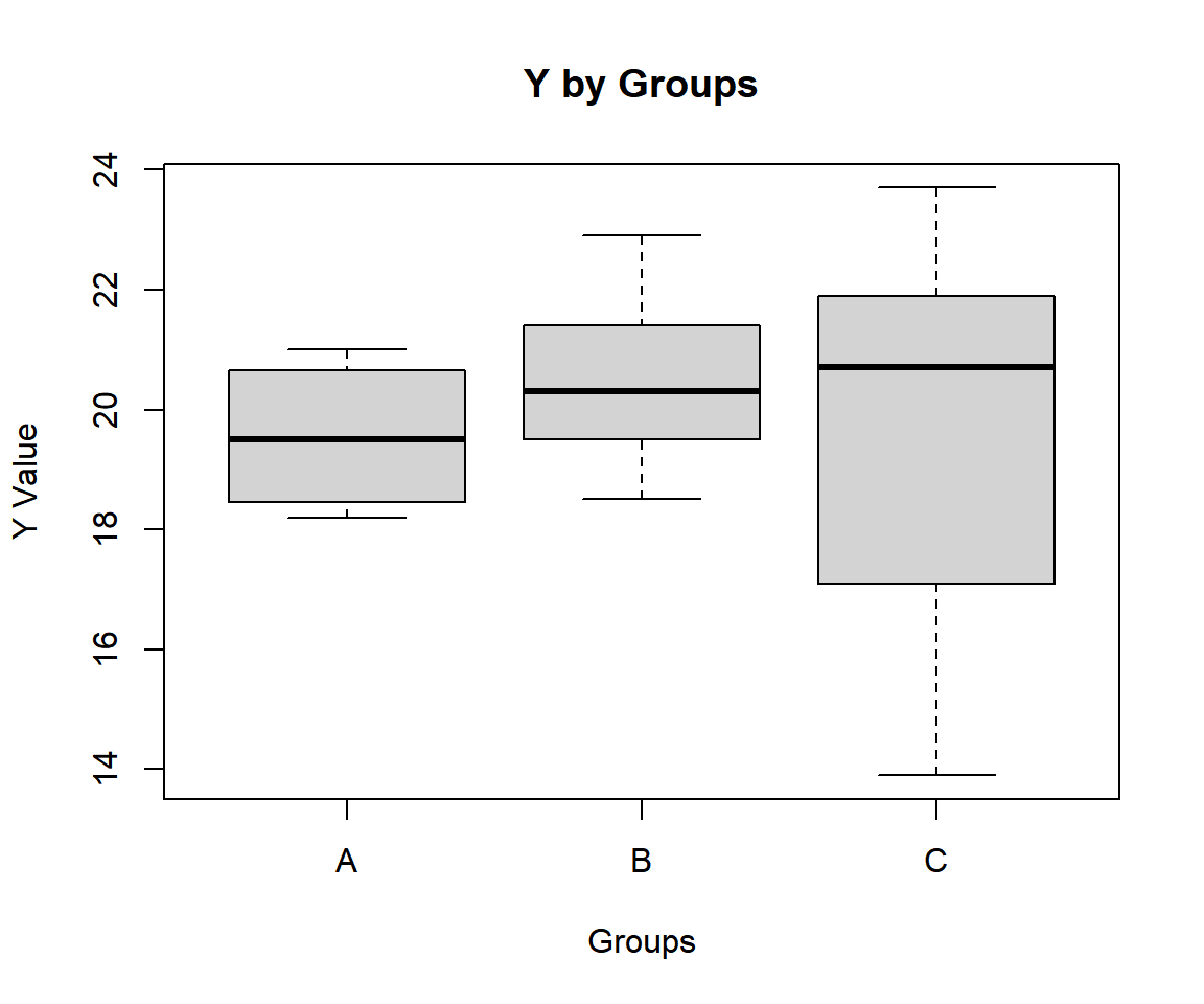
Simple One-way ANOVA Test Box Plot in R

The group and overall means, variances and lengths are:

c(tapply(y, groups, mean), mean(y))

       A        B        C          
19.55000 20.48333 19.46000 19.89333

c(tapply(y, groups, var), var(y))

        A         B         C           
 1.736667  2.585667 15.488000  5.970667

c(tapply(y, groups, length), length(y))

 A  B  C    
 4  6  5 15

For the following null hypothesis $H_0$, and alternative hypothesis $H_1$, with the level of significance $\alpha=0.05$.

$H_0:$ the group population means are equal ($\mu_A = \mu_B = \mu_C$).

$H_1:$ at least one group’s mean is different from the rest.

anova(lm(y ~ groups))

Analysis of Variance Table

Response: y
          Df Sum Sq Mean Sq F value Pr(>F)
groups     2  3.499  1.7495  0.2621 0.7737
Residuals 12 80.090  6.6742

Or:

oneway.test(y ~ groups, var.equal = TRUE)


    One-way analysis of means

data:  y and groups
F = 0.26213, num df = 2, denom df = 12, p-value = 0.7737

The test statistic, $F$, is 0.26213,

the degrees of freedom, are numerator df $G-1= 2$, denominator df $N-G= 12$,

the p-value, $p$, is 0.7737.

Interpretation:

P-value: With the p-value ($p = 0.7737$) being greater than the level of significance 0.05, we fail to reject the null hypothesis that the group population means are equal.
$F$ T-statistic: With test statistics value ($F_{2, 12} = 0.26213$) being less than the critical value, $F_{2, 12, \alpha}=\text{qf(0.95, 2, 12)}$$=3.8852938$ (or not in the shaded region), we fail to reject the null hypothesis that the group population means are equal.

x = seq(0.01, 5, 1/1000); y = df(x, df1=2, df2=12)
plot(x, y, type = "l",
     xlim = c(0, 5), ylim = c(-0.06, min(max(y), 1)),
     main = "One-way ANOVA Test
Shaded Region for Simple Test",
     xlab = "x", ylab = "Density",
     lwd = 2, col = "blue")
abline(h=0)
# Add shaded region and legend
point = qf(0.95, 2, 12)
polygon(x = c(x[x >= point], 5, point),
        y = c(y[x >= point], 0, 0),
        col = "blue")
legend("topright", c("Area = 0.05"),
       fill = c("blue"), inset = 0.01)
# Add critical value and F-value
arrows(2.5, 0.4, 0.26213, 0)
text(2.5, 0.45, "F = 0.26213")
text(3.885294, -0.04, expression(F[alpha]==3.885294))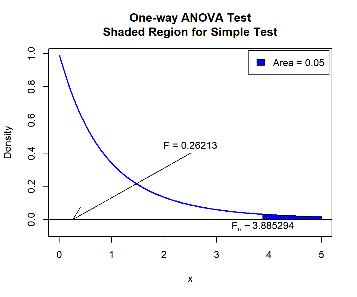

One-way ANOVA Test Shaded Region for Simple Test in R

See line charts, shading areas under a curve, lines & arrows on plots, mathematical expressions on plots, and legends on plots for more details on making the plot above.

3 One-way ANOVA Test Critical Value in R

To get the critical value for a one-way ANOVA test in R, you can use the qf() function for F-distribution to derive the quantile associated with the given level of significance value $\alpha$.

The critical value is qf($1-\alpha$, df1, df2).

Example:

For $\alpha = 0.1$, $\text{df1} = 3$, and $\text{df2} = 18$.

qf(0.9, 3, 18)

[1] 2.416005

4 One-way ANOVA Test in R

Using the PlantGrowth data from the "datasets" package with 10 sample rows from 30 rows below:

PlantGrowth

   weight group
1    4.17  ctrl
4    6.11  ctrl
5    4.50  ctrl
7    5.17  ctrl
12   4.17  trt1
17   6.03  trt1
19   4.32  trt1
20   4.69  trt1
23   5.54  trt2
30   5.26  trt2

Check variability between and within groups with a boxplot.

boxplot(weight ~ group, data = PlantGrowth,
     main = "Y by Groups",
     xlab = "Groups",
     ylab = "Y Value")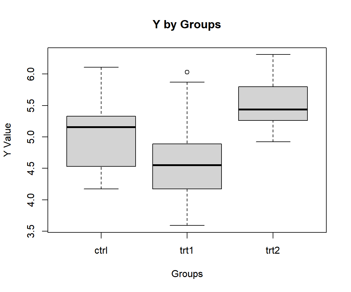

One-way ANOVA Test Box Plot in R

The group and overall means, variances and lengths are:

y = PlantGrowth$weight; x = PlantGrowth$group
c(tapply(y, x, mean), mean(y))

 ctrl  trt1  trt2       
5.032 4.661 5.526 5.073

c(tapply(y, x, var), var(y))

     ctrl      trt1      trt2           
0.3399956 0.6299211 0.1958711 0.4916700

c(tapply(y, x, length), length(y))

ctrl trt1 trt2      
  10   10   10   30

For the following null hypothesis $H_0$, and alternative hypothesis $H_1$, with the level of significance $\alpha=0.1$.

$H_0:$ the group population means are equal ($\mu_{ctrl} = \mu_{trt1} = \mu_{trt2}$).

$H_1:$ at least one group’s mean is different from the rest.

anova(lm(weight ~ group, data = PlantGrowth))

Analysis of Variance Table

Response: weight
          Df  Sum Sq Mean Sq F value  Pr(>F)  
group      2  3.7663  1.8832  4.8461 0.01591 *
Residuals 27 10.4921  0.3886                  
---
Signif. codes:  0 '***' 0.001 '**' 0.01 '*' 0.05 '.' 0.1 ' ' 1

Or:

oneway.test(weight ~ group, data = PlantGrowth,
            var.equal = TRUE)


    One-way analysis of means

data:  weight and group
F = 4.8461, num df = 2, denom df = 27, p-value = 0.01591

Interpretation:

P-value: With the p-value ($p = 0.01591$) being less than the level of significance 0.1, we reject the null hypothesis that the group population means are equal.
$F$ T-statistic: With test statistics value ($F_{2, 27} = 4.8461$) being in the critical region (shaded area), that is, $F_{2, 27} = 4.8461$ greater than $F_{2, 27, \alpha}=\text{qf(0.9, 2, 27)}$$=2.5106087$, we reject the null hypothesis that the group population means are equal.

x = seq(0.01, 5, 1/1000); y = df(x, df1=2, df2=27)
plot(x, y, type = "l",
     xlim = c(0, 5), ylim = c(-0.06, max(y)),
     main = "One-way ANOVA Test
Shaded Region",
     xlab = "x", ylab = "Density",
     lwd = 2, col = "blue")
abline(h=0)
# Add shaded region and legend
point = qf(0.9, 2, 27)
polygon(x = c(x[x >= point], 5, point),
        y = c(y[x >= point], 0, 0),
        col = "blue")
legend("topright", c("Area = 0.1"),
       fill = c("blue"), inset = 0.01)
# Add critical value and F-value
arrows(4, 0.3, 4.8461, 0)
text(4, 0.35, expression(F==4.8461))
text(2.510609, -0.04, expression(F[alpha]==2.510609))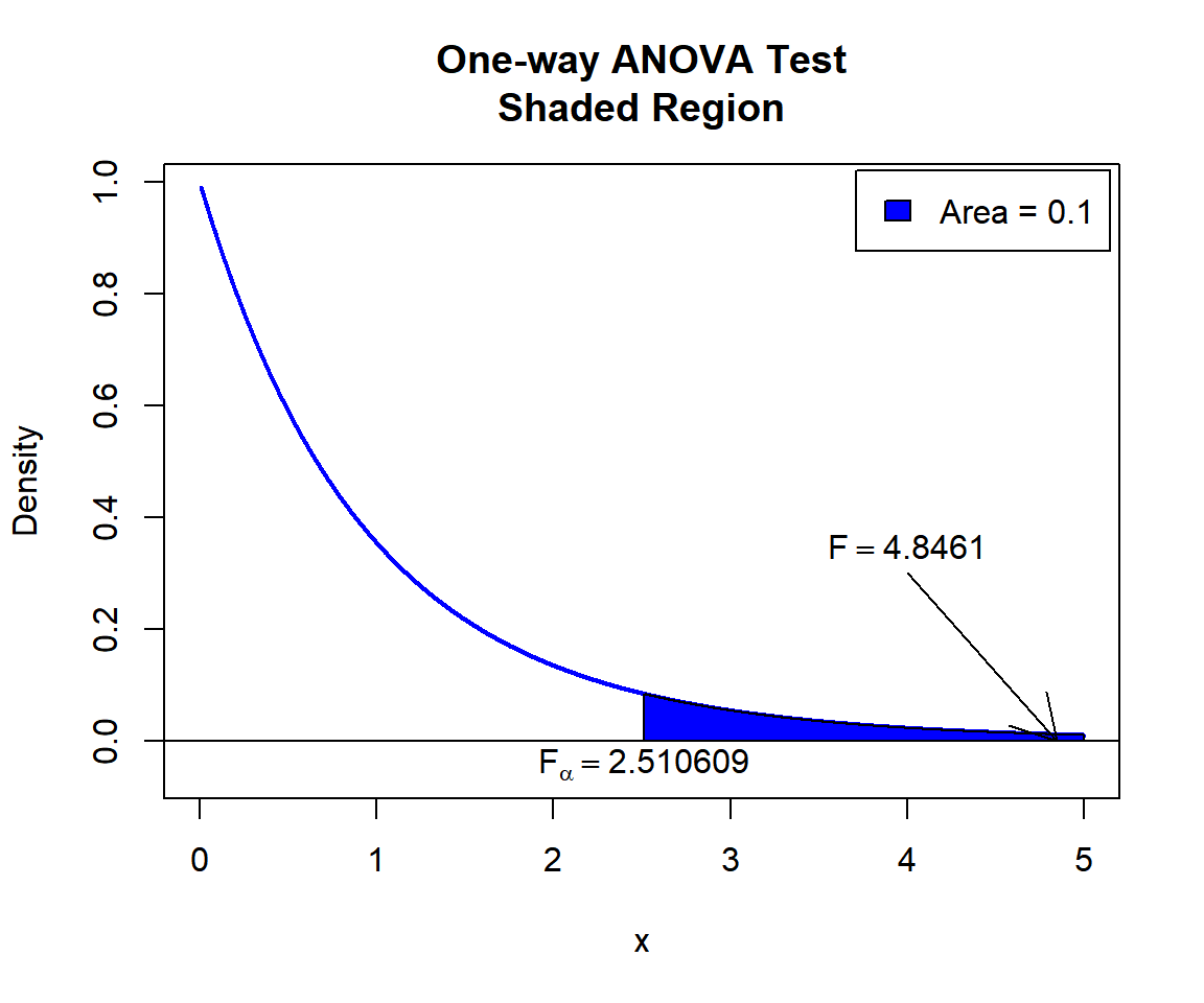

One-way ANOVA Test Shaded Region in R

5 One-way ANOVA Test: Test Statistics, P-value & Degrees of Freedom in R

Here for a one-way ANOVA test, we show how to get the test statistics (or f-value), sum of squares, mean squares, p-values, and degrees of freedom from the anova() or oneway.test() function in R, or by written code.

aov_object = anova(lm(weight ~ feed, data = chickwts))
owt_object = oneway.test(weight ~ feed, data = chickwts,
                          var.equal = TRUE)
aov_object

Analysis of Variance Table

Response: weight
          Df Sum Sq Mean Sq F value    Pr(>F)    
feed       5 231129   46226  15.365 5.936e-10 ***
Residuals 65 195556    3009                      
---
Signif. codes:  0 '***' 0.001 '**' 0.01 '*' 0.05 '.' 0.1 ' ' 1

owt_object


    One-way analysis of means

data:  weight and feed
F = 15.365, num df = 5, denom df = 65, p-value = 5.936e-10

To get the test statistic (or f-value), sum of squares, and mean squares:

F-value

\[\begin{align*} F & = \frac{\left[ \sum_{j=1}^G N_j(\bar y_{j\cdot}-\bar y_{\cdot \cdot})^2 \right] / (G-1)}{\left[ \sum_{j=1}^G \sum_{k=1}^{N_j} (y_{jk}-\bar y_{j\cdot})^2 \right]/ (N-G)}\\ & = \frac{\left[ \sum_{j=1}^G N_j(\bar y_{j.}-\bar y_{\cdot \cdot})^2 \right]/ (G-1)}{\left[ \sum_{j=1}^G (N_j-1) s_j^2 \right]/ (N-G)}. \end{align*}\]

aov_object$`F value`[1]

[1] 15.3648

owt_object$statistic

      F 
15.3648

# to remove name F
unname(owt_object$statistic)

[1] 15.3648

Same as:

# Method 1
y = chickwts$weight; group = chickwts$feed
f_order = order(group); y = y[f_order]; group = group[f_order] #order by group
means = tapply(y, group, mean) #means
lens = tapply(y, group, length) #sizes
G = length(unique(group)); N = length(y) #lengths
ssg = sum(lens*(means-mean(y))^2) #sums of squares
ssr = sum((y-rep(means, lens))^2)
num = ssg/(G-1); denom = ssr/(N-G) #mean squares
F = num/denom
F

[1] 15.3648

# Method 2
y = chickwts$weight; group = chickwts$feed
means = tapply(y, group, mean) #means
vars = tapply(y, group, var) #variances
lens = tapply(y, group, length) #sizes
G = length(unique(group)); N = length(y) #lengths
ssg = sum(lens*(means-mean(y))^2) #sums of squares
ssr = sum((lens-1)*vars)
num = ssg/(G-1); denom = ssr/(N-G) #mean squares
F = num/denom
F

[1] 15.3648

Sum of squares and mean squares

aov_object$`Sum Sq`

[1] 231129.2 195556.0

aov_object$`Mean Sq`

[1] 46225.832  3008.554

Same as (based on steps above):

c(ssg, ssr)

[1] 231129.2 195556.0

c(num, denom)

[1] 46225.832  3008.554

To get the p-value:

The p-value is, $P (F_{df1, df2}>F_{Observed})$

aov_object$`Pr(>F)`[1]

[1] 5.93642e-10

owt_object$p.value

[1] 5.93642e-10

Same as:

Note that the p-value depends on the $\text{test statistics}$ ($F_{df1, df2} = 15.3648$), and $\text{degrees of freedom}$ (5, 65). We also use the distribution function pf() for the F distribution in R.

1-pf(15.3648, 5, 65)

[1] 5.936418e-10

To get the degrees of freedom:

The degrees of freedom are $\text{df1}=5$ and $\text{df2}=65$.

aov_object$Df

[1]  5 65

owt_object$parameter

  num df denom df 
       5       65

# to remove names num df, denom df
unname(owt_object$parameter)

[1]  5 65

Same as:

G = length(unique(group)); N = length(y)
c(G-1, N-G)

[1]  5 65

Source of Variation	Degrees of Freedom (DF)	Sums of Squares (SS)	Mean Square (MS)	F	P-value
Groups	\(G-1\)	\(\sum_{j=1}^G N_j(\bar y_{j\cdot}-\bar y_{\cdot \cdot})^2\)	\(\frac{SS_{groups}}{DF_{groups}}\)	\(\frac{MS_{groups}}{MS_{residuals}}\)	\(P(F_{G-1,N-G}>F)\)
Residuals	\(N-G\)	\(\sum_{j=1}^G \sum_{k=1}^{N_j} (y_{jk}-\bar y_{j\cdot})^2\)	\(\frac{SS_{residuals}}{DF_{residuals}}\)
Total	\(N-1\)	\(\sum_{j=1}^G \sum_{k=1}^{N_j} (y_{jk}-\bar y_{\cdot \cdot})^2\)

Question	Are the group means equal?
Null Hypothesis, \(H_0\)	\(\mu_1 = \mu_2 = \dots = \mu_G\)
Alternate Hypothesis, \(H_1\)	At least one group’s mean is different from the rest.

One-way ANOVA Tests in R

Sample Steps to Run a One-way ANOVA Test:

Creating a One-way ANOVA Test Object:

1 Test Statistic for One-way ANOVA Test in R

2 Simple One-way ANOVA Test in R

Interpretation:

3 One-way ANOVA Test Critical Value in R

4 One-way ANOVA Test in R

Interpretation:

5 One-way ANOVA Test: Test Statistics, P-value & Degrees of Freedom in R

To get the test statistic (or f-value), sum of squares, and mean squares:

F-value

Sum of squares and mean squares

To get the p-value:

To get the degrees of freedom: