1 Table of Weibull Distribution Functions in R
2 Plot of Weibull Distributions in R
3 Examples for Setting Parameters for Weibull Distributions in R
4 rweibull(): Random Sampling from Weibull Distributions in R
5 dweibull(): Probability Density Function for Weibull Distributions in R
6 pweibull(): Cumulative Distribution Function for Weibull Distributions in R
7 qweibull(): Derive Quantile for Weibull Distributions in R

Here, we discuss Weibull distribution functions in R, plots, parameter setting, random sampling, density, cumulative distribution and quantiles.

The Weibull distribution with parameters \(\tt{shape}=\alpha\), and \(\tt{scale}=\lambda\) has probability density function (pdf) formula as:

\[ f(x) = \begin{cases} \frac{\alpha}{\lambda}\left(\frac{x}{\lambda}\right)^{\alpha-1}e^{-(x/\lambda)^\alpha}, & x\ge0,\\ 0 \;, & x<0,\end{cases}\]

where \(\alpha>0\), and \({\lambda>0}\).

The mean is \(\lambda \, \Gamma(1+1/\alpha)\,\), and the variance is \(\lambda^2\left[\Gamma\left(1+\frac{2}{\alpha}\right) - \left(\Gamma\left(1+\frac{1}{\alpha}\right)\right)^2\right]\), where \(\Gamma\) is the \(\tt{gamma\;function}\).

1 Table of Weibull Distribution Functions in R

The table below shows the functions for Weibull distributions in R.

Table of Weibull Distribution Functions in R
Function	Usage
rweibull(n, shape, scale=1)	Simulate a random sample with \(n\) observations
dweibull(x, shape, scale=1)	Calculate the probability density at the point \(x\)
pweibull(q, shape, scale=1)	Calculate the cumulative distribution at the point \(q\)
qweibull(p, shape, scale=1)	Calculate the quantile value associated with \(p\)

2 Plot of Weibull Distributions in R

Single distribution:

Below is a plot of the Weibull distribution function with \(\tt{shape}=2.5\) and \(\tt{scale}=3\).

x = seq(0, 8, 1/1000); y = dweibull(x, 2.5, 3)
plot(x, y, type = "l",
     xlim = c(0, 8), ylim = c(0, max(y)),
     main = "Probability Density Function of Weibull Distribution (2.5, 3)",
     xlab = "x", ylab = "Density",
     lwd = 2, col = "blue")
# Add legend
legend("topright", "shape = 2.5 \nscale = 3",
       lwd = 2,
       col = "blue",
       bty = "n")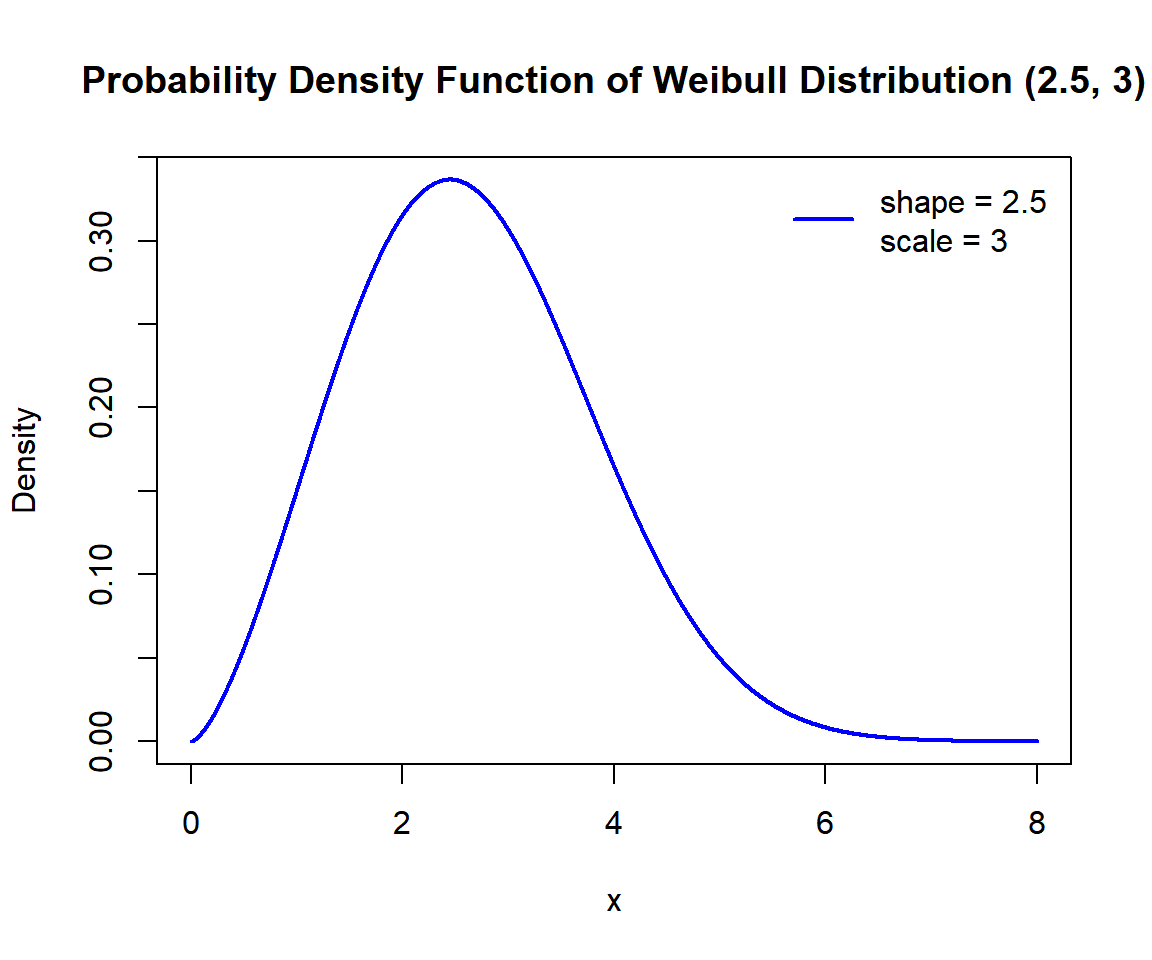

Probability Density Function (PDF) of a Weibull Distribution in R

Multiple distributions:

Below is a plot of multiple Weibull distribution functions in one graph.

x1 = seq(0, 7, 1/1000); y1 = dweibull(x1, 3, 1)
x2 = seq(0, 7, 1/1000); y2 = dweibull(x2, 1, 1)
x3 = seq(0, 7, 1/1000); y3 = dweibull(x3, 1, 2)
x4 = seq(0.05, 7, 1/1000); y4 = dweibull(x4, 0.5, 2)
plot(x1, y1, type = "l",
     xlim = c(0, 7), ylim = range(c(y1, y2, y3, y4)),
     main = "Probability Density Functions of Weibull Distributions",
     xlab = "x", ylab = "Density",
     lwd = 2, col = "blue")
points(x2, y2, type = "l", lwd = 2, col = "red")
points(x3, y3, type = "l", lwd = 2, col = "green")
points(x4, y4, type = "l", lwd = 2, col = "black")
# Add legend
legend("topright", c("shape = 3,    scale = 1",
                    "shape = 1,    scale = 1",
                    "shape = 1,    scale = 2",
                    "shape = 0.5, scale = 2"),
       lwd = c(2, 2, 2, 2),
       col = c("blue", "red", "green", "black"),
       bty = "n")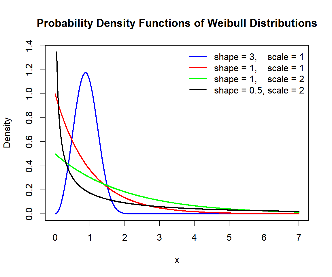

Probability Density Functions (PDFs) of Weibull Distributions in R

3 Examples for Setting Parameters for Weibull Distributions in R

In the Weibull distribution functions, the scale parameter is pre-specified as \(\lambda=1\), hence it does not need to be specified, unless it is to be set to a different value.

For example, for dweibull(), the following are the same:

# The order of 2 and 1 matters here as the parameter names are not used.
# The first number 2 is shape, and 1 is scale.
dweibull(0.3, 2); dweibull(0.3, 2, 1)

[1] 0.5483587

[1] 0.5483587

# Or:
dweibull(0.3, shape = 2, scale = 1)

[1] 0.5483587

# Or:
dweibull(0.3, scale = 1, shape = 2)

[1] 0.5483587

4 rweibull(): Random Sampling from Weibull Distributions in R

Sample 1200 observations from the Weibull distribution with \(\tt{shape} = 1.2\) and \(\tt{scale} = 4\):

rweibull(1200, 1.2, 4)

set.seed(100) # Line allows replication (use any number).
sample = rweibull(1200, 1.2, 4)
hist(sample,
     main = "Histogram of 1200 Observations from Weibull Distribution
with Shape = 1.2 and Scale = 4",
     xlab = "x",
     col = "deepskyblue", border = "white")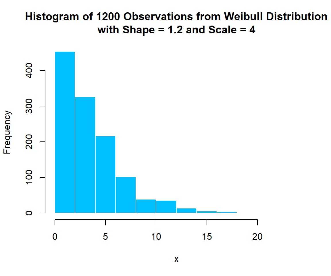

Histogram of Weibull Distribution (1.2, 4) Random Sample in R

5 dweibull(): Probability Density Function for Weibull Distributions in R

Calculate the density at \(x = 0.65\), in the Weibull distribution with \(\tt{shape} = 0.7\) and \(\tt{scale} = 2.4\):

dweibull(0.65, 0.7, 2.4)

[1] 0.2890849

x = seq(0.1, 9, 1/1000); y = dweibull(x, 0.7, 2.4)
plot(x, y, type = "l",
     xlim = c(0, 9), ylim = c(0, max(y)),
     main = "Probability Density Function of Weibull Distribution
with Shape = 0.7 and Scale = 2.4",
     xlab = "x", ylab = "Density",
     lwd = 2, col = "blue")
# Add lines
segments(0.65, -1, 0.65, 0.2890849)
segments(-1, 0.2890849, 0.65, 0.2890849)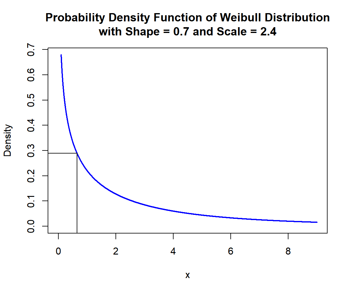

Probability Density Function (PDF) of Weibull Distribution (0.7, 2.4) in R

6 pweibull(): Cumulative Distribution Function for Weibull Distributions in R

Calculate the cumulative distribution at \(x = 3.1\), in the Weibull distribution with \(\tt{shape} = 1.4\) and \(\tt{scale} = 2\). That is, \(P(X \le 3.1)\):

pweibull(3.1, 1.4, 2)

[1] 0.8422887

x = seq(0, 8, 1/1000); y = pweibull(x, 1.4, 2)
plot(x, y, type = "l",
     xlim = c(0, 8), ylim = c(0,1),
     main = "Cumulative Distribution Function of Weibull Distribution
with Shape = 1.4 and Scale = 2",
     xlab = "x", ylab = "Cumulative Distribution",
     lwd = 2, col = "blue")
# Add lines
segments(3.1, -1, 3.1, 0.8422887)
segments(-6, 0.8422887, 3.1, 0.8422887)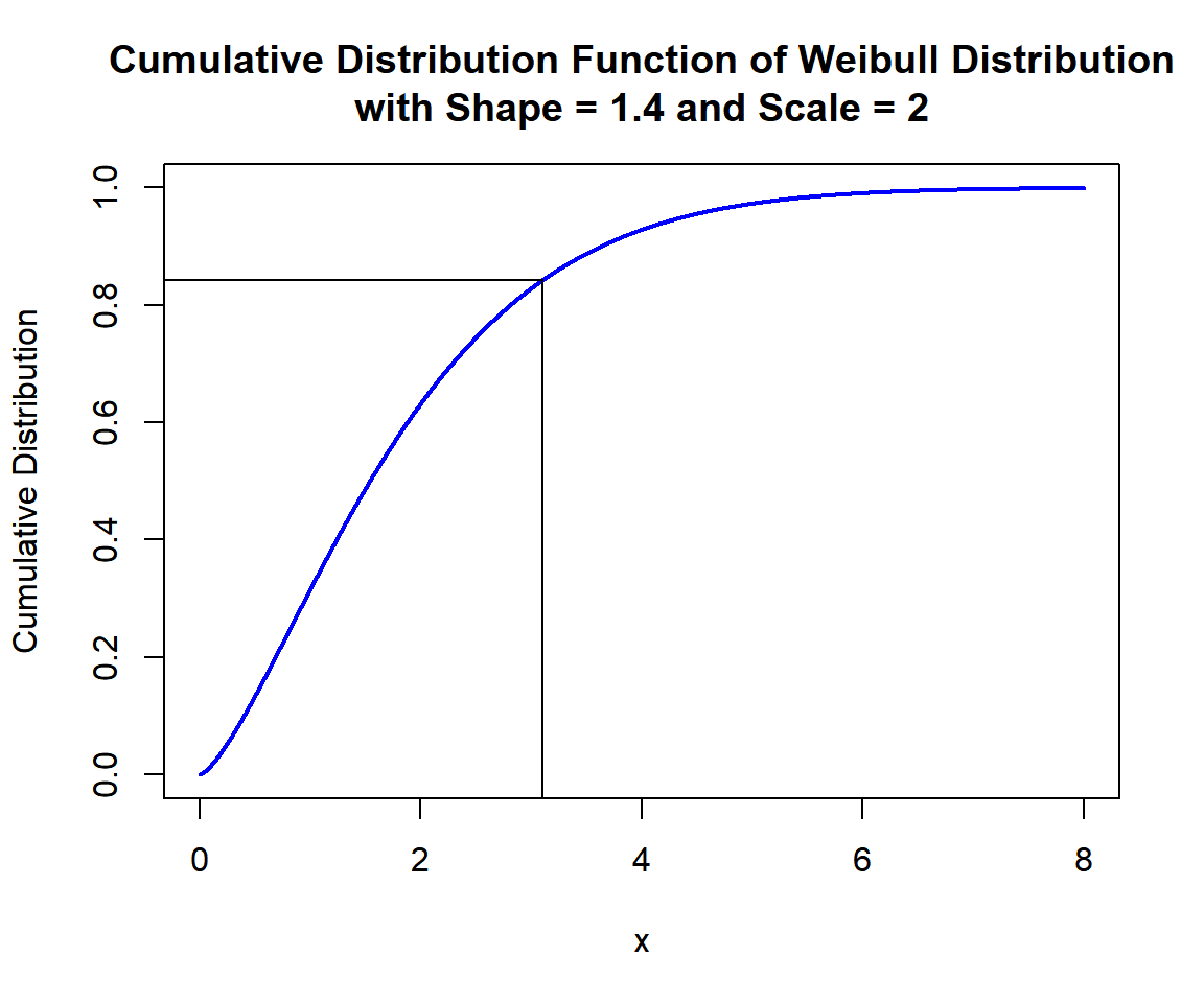

Cumulative Distribution Function (CDF) of Weibull Distribution (1.4, 2) in R

x = seq(0, 8, 1/1000); y = dweibull(x, 1.4, 2)
plot(x, y, type = "l",
     xlim = c(0, 8), ylim = c(0, max(y)),
     main = "Probability Density Function of Weibull Distribution
with Shape = 1.4 and Scale = 2",
     xlab = "x", ylab = "Density",
     lwd = 2, col = "blue")
# Add shaded region and legend
point = 3.1
polygon(x = c(x[x <= point], point),
        y = c(y[x <= point], 0),
        col = "limegreen")
legend("topright", c("Area = 0.8422887"),
       fill = c("limegreen"),
       inset = 0.01)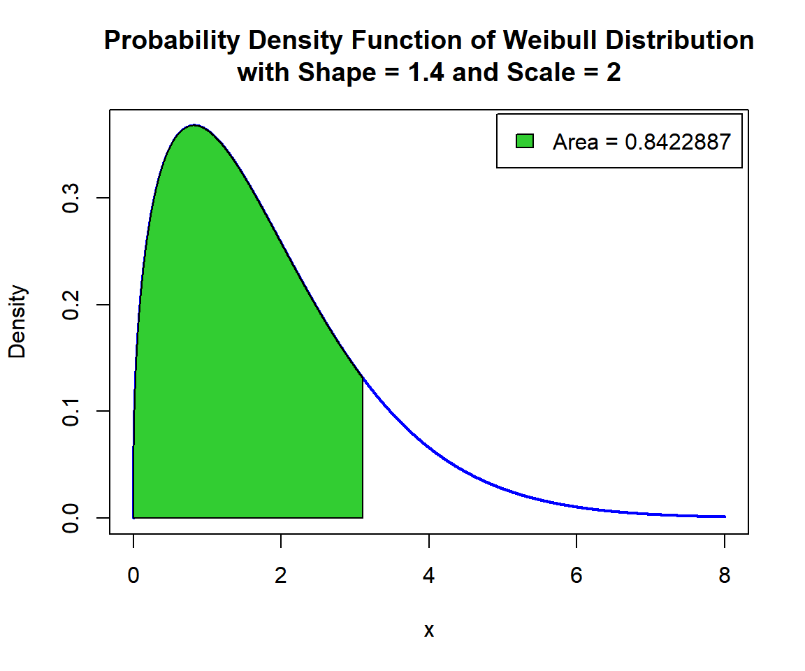

Shaded Probability Density Function (PDF) of Weibull Distribution (1.4, 2) in R

For upper tail, at \(x = 3.1\), that is, \(P(X \ge 3.1) = 1 - P(X \le 3.1)\), set the "lower.tail" argument:

pweibull(3.1, 1.4, 2, lower.tail = FALSE)

[1] 0.1577113

x = seq(0, 8, 1/1000); y = dweibull(x, 1.4, 2)
plot(x, y, type = "l",
     xlim = c(0, 8), ylim = c(0, max(y)),
     main = "Shaded Upper Region: Probability Density Function of
Weibull Distribution with Shape = 1.4 and Scale = 2",
     xlab = "x", ylab = "Density",
     lwd = 2, col = "blue")
# Add shaded region and legend
point = 3.1
polygon(x = c(point, x[x >= point]),
        y = c(0, y[x >= point]),
        col = "limegreen")
legend("topright", c("Area = 0.1577113"),
       fill = c("limegreen"),
       inset = 0.01)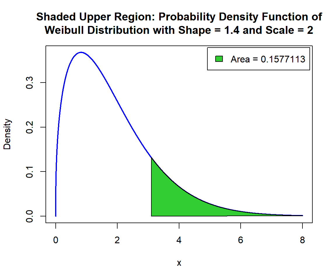

Shaded Upper Region: Probability Density Function (PDF) of Weibull Distribution (1.4, 2) in R

7 qweibull(): Derive Quantile for Weibull Distributions in R

Derive the quantile for \(p = 0.9\), in the Weibull distribution with \(\tt{shape} = 3\) and \(\tt{scale} = 2\). That is, \(x\) such that, \(P(X \le x)=0.9\):

qweibull(0.9, 3, 2)

[1] 2.641001

x = seq(0, 4, 1/1000); y = pweibull(x, 3, 2)
plot(x, y, type = "l",
     xlim = c(0, 4), ylim = c(0,1),
     main = "Cumulative Distribution Function of Weibull Distribution
with Shape = 3 and Scale = 2",
     xlab = "x", ylab = "Cumulative Distribution",
     lwd = 2, col = "blue")
# Add lines
segments(2.641001, -1, 2.641001, 0.9)
segments(-1, 0.9, 2.641001, 0.9)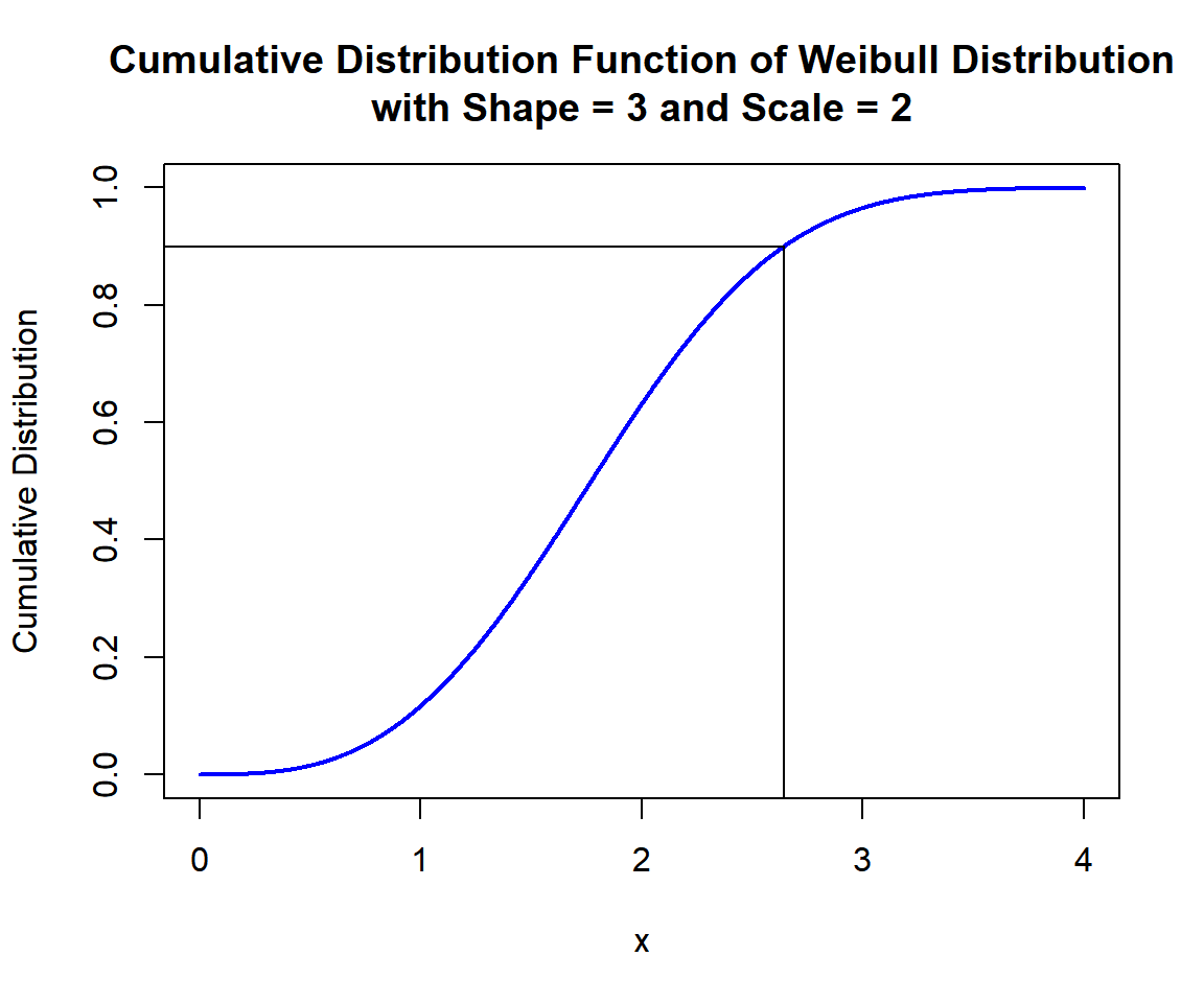

Cumulative Distribution Function (CDF) of Weibull Distribution (3, 2) in R

x = seq(0, 4, 1/1000); y = dweibull(x, 3, 2)
plot(x, y, type = "l",
     xlim = c(0, 4), ylim = c(0, max(y)),
     main = "Probability Density Function of Weibull Distribution
with Shape = 3 and Scale = 2",
     xlab = "x", ylab = "Density",
     lwd = 2, col = "blue")
# Add shaded region and legend
point = 2.641001
polygon(x = c(x[x <= point], point),
        y = c(y[x <= point], 0),
        col = "limegreen")
legend("topright", c("Area = 0.9"),
       fill = c("limegreen"),
       inset = 0.01)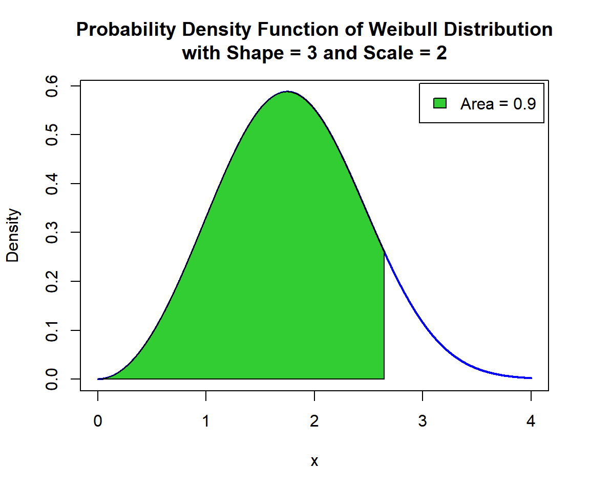

Shaded Probability Density Function (PDF) of Weibull Distribution (3, 2) in R

For upper tail, for \(p = 0.1\), that is, \(x\) such that, \(P(X \ge x)=0.1\):

qweibull(0.1, 3, 2, lower.tail = FALSE)

[1] 2.641001

x = seq(0, 4, 1/1000); y = dweibull(x, 3, 2)
plot(x, y, type = "l",
     xlim = c(0, 4), ylim = c(0, max(y)),
     main = "Shaded Upper Region: Probability Density Function of
Weibull Distribution with Shape = 3 and Scale = 2",
     xlab = "x", ylab = "Density",
     lwd = 2, col = "blue")
# Add shaded region and legend
point = 2.641001
polygon(x = c(point, x[x >= point]),
        y = c(0, y[x >= point]),
        col = "limegreen")
legend("topright", c("Area = 0.1"),
       fill = c("limegreen"),
       inset = 0.01)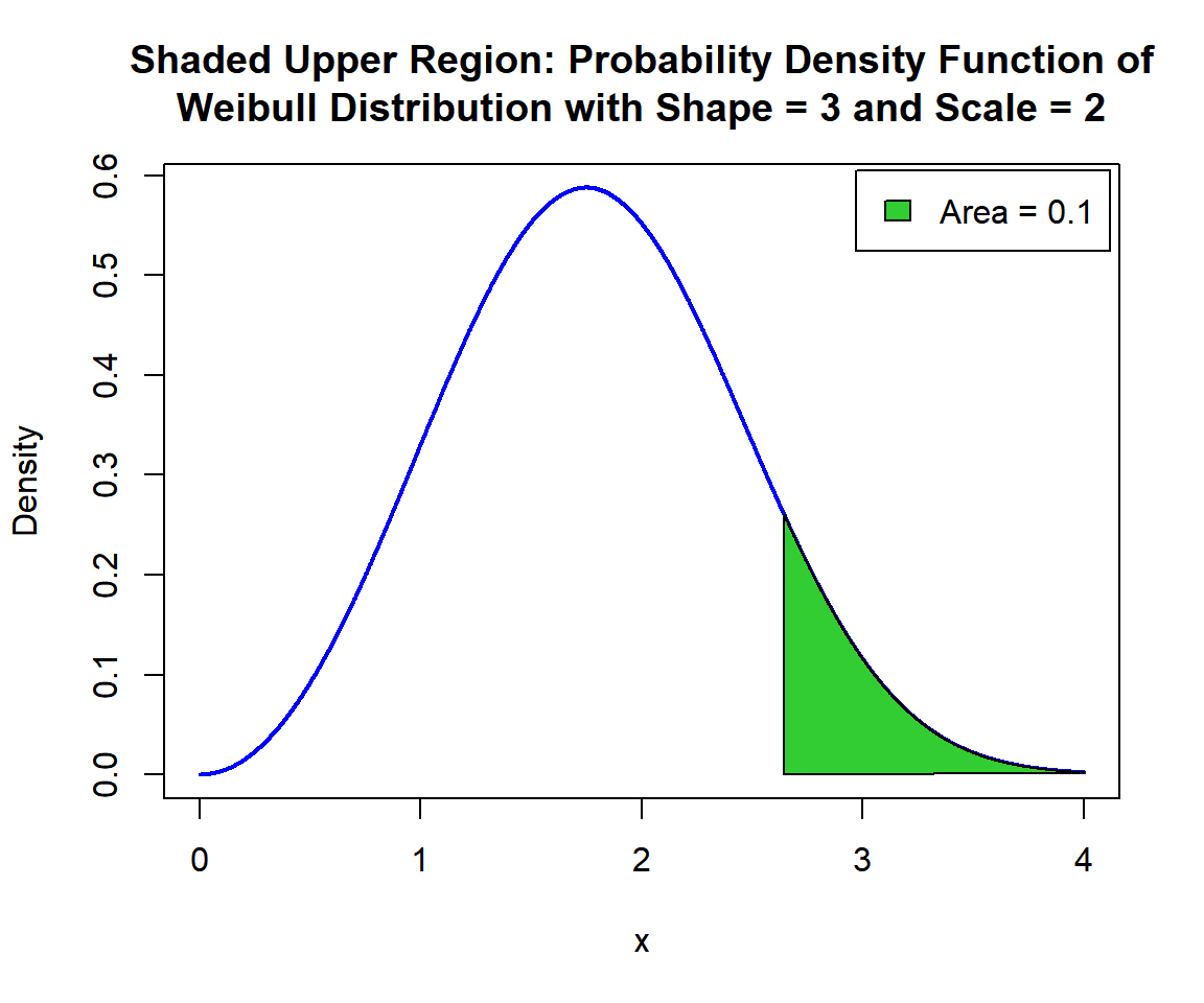

Shaded Upper Region: Probability Density Function (PDF) of Weibull Distribution (3, 2) in R