Shade Areas and Regions, Between Points, Under Curves & Above Curves in R
Here we discuss how to shade areas and regions on plots in R: shading area under or above a curve, and shading area between points or area between curves.
This will be done using the polygon() function from the
"graphics" package.
| Argument | Usage |
| col | Set shade fill color |
| density | Set shade line density |
| lty | Set shade line type |
| angle | Set shade line angle |
See also texts on plots, point types & sizes, line types & widths, lines & segments on plots, setting colors & fonts, plotting curves, and mathematical expressions on plots.
1 Shade Area Between Points on Plots & Charts in R
Here we show how to shade the area between points using the
polygon() function.
Simple Area
Points to which area within is to be shaded:
Triangular area with points (2, 8) to (0, 2) to (4, 2), and rectangular area with points (6, 8) to (6, 2) to (10, 2) to (10, 8).
plot(12, 10, pch = "",
     xlim = c(-0.5, 12), ylim = c(0,10),
     xlab = "", ylab = "",
     main = "Points to Shade Area Between")

# Triangular points
points(c(2, 0, 4), y = c(8, 2, 2), col = "blue")
text(2, 8, "(2, 8)", adj = c(0.5, -1))
text(0, 2, "(0, 2)", adj = c(0.5, 1.5))
text(4, 2, "(4, 2)", adj = c(0.5, 1.5))

# Rectangular points
points(c(6, 6, 10, 10), y = c(8, 2, 2, 8), col = "red")
text(6, 8, "(6, 8)", adj = c(0.5, -1))
text(6, 2, "(6, 2)", adj = c(0.5, 1.5))
text(10, 2, "(10, 2)", adj = c(0.5, 1.5))
text(10, 8, "(10, 8)", adj = c(0.5, -1))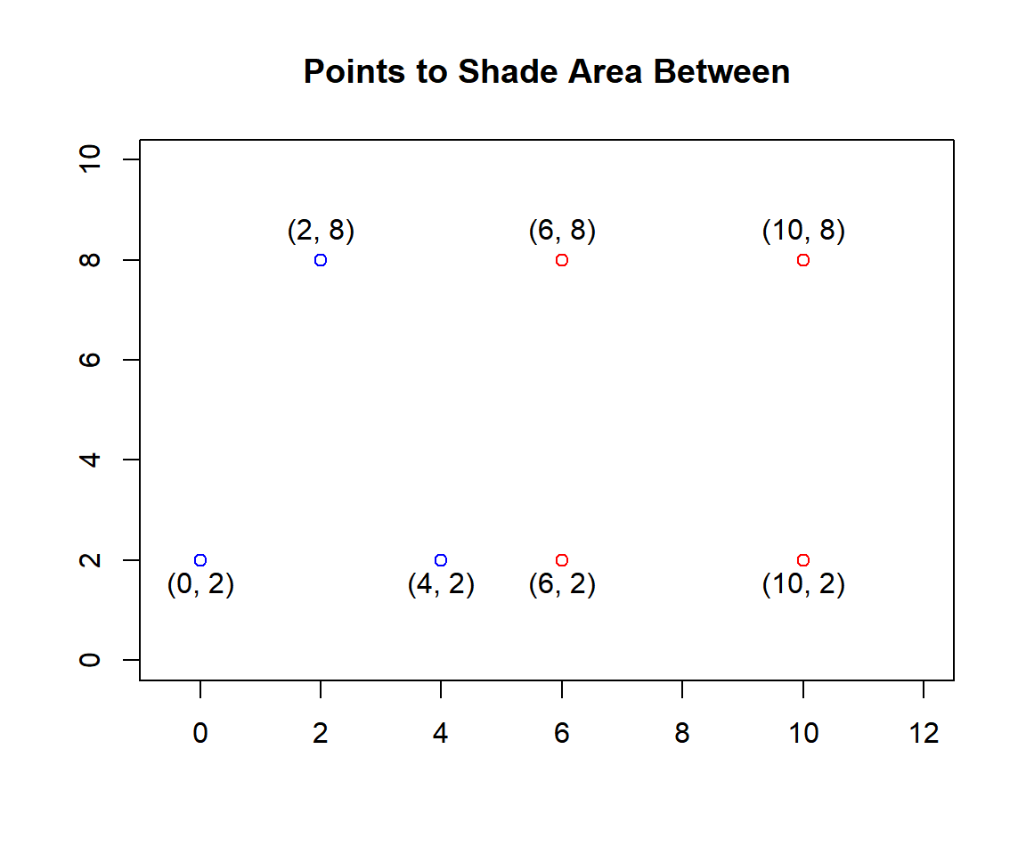
Points to Shade Area Between in R
With the points highlighted, join the points and shade the area between with the following codes:
The function draws a line between points in the order set, draws the last line from the last point to the first point, and then shades the enclosed area.
# Specify the three x and y triangular points in enclosing order.
polygon(x = c(2, 0, 4), y = c(8, 2, 2),
        col = "blue")

# Specify the four x and y rectangular points in enclosing order.
polygon(x = c(6, 6, 10, 10), y = c(8, 2, 2, 8),
        col = "red",
        density = 10, lty = 4, angle = 45)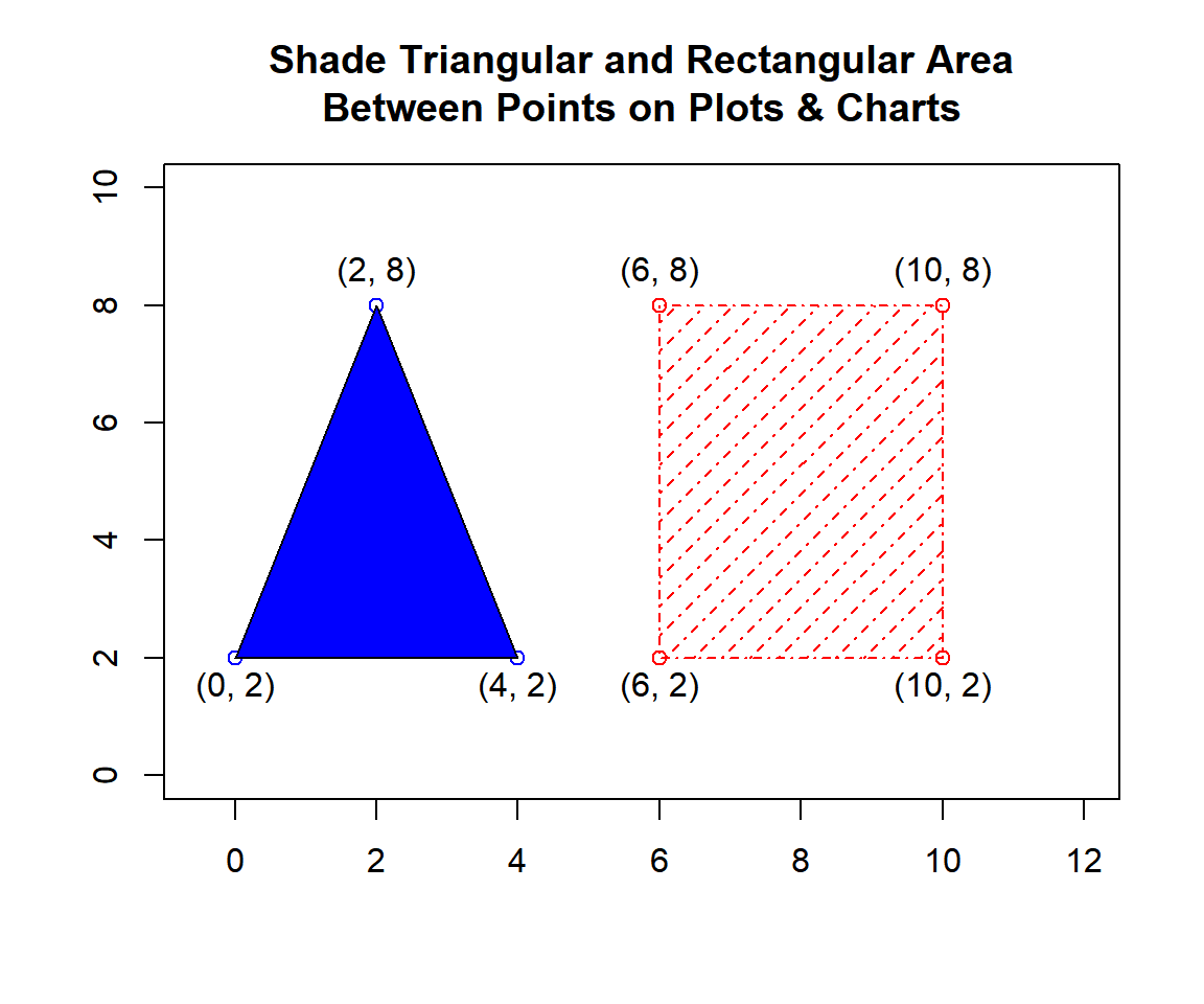
Shade Triangular and Rectangular Area Between Points on Plots & Charts in R
Complex Area
To shade complex areas between points, set the x and y points in the enclosing order as in the examples below:
Points (0, 8) to (4, 8) to (0, 2) to (4, 2), then the function draws back to (0, 8) and shades enclosed area.
Points (6, 8) to (6, 2) to (10, 8) to (12, 5) to (10, 2), then the function draws back to (6, 8) and shades enclosed area.
plot(12, 10, pch = "",
     xlim = c(-0.5, 12.5), ylim = c(0,10),
     xlab = "", ylab = "",
     main = "Shade Complex Area Between Points on Plots & Charts")

# Blue lines: specify the x and y points in enclosing order.
polygon(x = c(0, 4, 0, 4), y = c(8, 8, 2, 2),
        col = "blue",
        density = 5, lty = 3, angle = 90)

# Red area: specify the x and y points in enclosing order.
polygon(x = c(6, 6, 10, 12, 10), y = c(8, 2, 8, 5, 2),
        col = "red")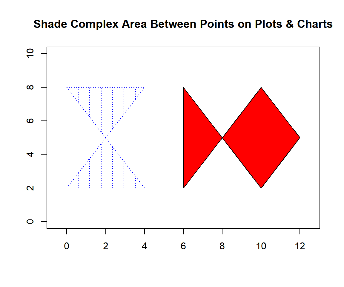
Shade Complex Area Between Points on Plots & Charts in R
2 Shade Area & Region Under a Curve in R
Here we show how to shade the area under a curve using the
polygon() function.
Area Under a Curve
Using the function \(y=x^3+x\) as an example.
To shade the area under the curve, start at the left point (0, 0), follow the curve, all (x, y)’s, up to (2, \(y = 2^3 + 2\)), down to (2, 0), then the function draws back to (0, 0) and shades enclosed area.
x = seq(0, 2, 1/100); y = (x^3)+x
plot(x, y, type = "l",
     main = "Shade Area Under a Curve")
abline(h = 0)
text(1, 5, expression(f(x) == x^3+x))

# Specify the x and y points in enclosing order.
polygon(x = c(0, x, 2, 2),
        y = c(0, y, (2^3)+2, 0),
        col = "blue")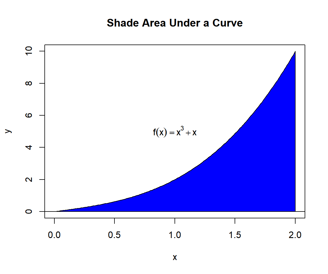
Shade Area Under a Curve in R
Region Under a Curve
Next, shaded regions under a curve using the function \(y=x^2\) as an example.
Shade regions: \(-0.8\leq x \leq -0.3\), and \(0 \leq x \leq 0.5\).
To shade the red region under the curve, start at the left bottom point (-0.8, 0), up to (-0.8, \(y = -0.8^2\)), follow the curve, all (x, y)’s for \(-0.8\leq x \leq -0.3\), down to (-0.3, \(y = -0.3^2\)), draw down to (-0.3, 0), then the function draws back to (-0.8, 0) and shades enclosed area.
To shade the green region under the curve, start at the left point (0, 0), follow the curve, all (x, y)’s for \(0 \leq x \leq 0.5\), up to (0.5, \(y = 0.5^2\)), down to (0.5, 0), then the function draws back to (0, 0) and shades enclosed area.
x = seq(-1, 1, 1/100); y = x^(2)
plot(x, y, type = "l",
     main = "Shade Regions Under a Curve")
abline(h = 0)
text(0, 0.5, expression(f(x) == x^2))

# Red area: specify the x and y points in enclosing order.
polygon(x = c(-0.8, -0.8, x[x>(-0.8) & x<(-0.3)], -0.3, -0.3),
        y = c(0, (-0.8)^2, y[x>(-0.8) & x<(-0.3)], (-0.3)^2, 0),
        col = "red")

# Green area: specify the x and y points in enclosing order.
polygon(x = c(0, x[x>0 & x<0.5], 0.5, 0.5),
        y = c(0, y[x>0 & x<0.5], 0.5^2, 0),
        col = "green")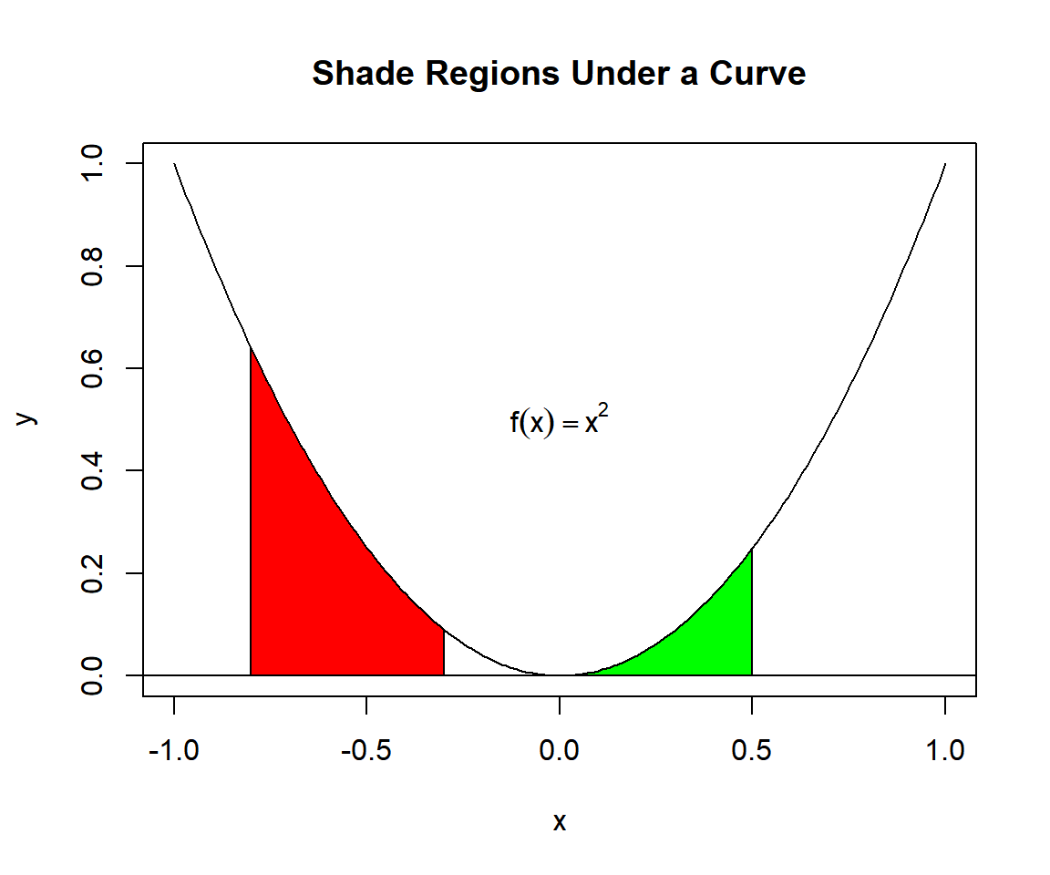
Shade Regions Under a Curve in R
3 Shade Area & Region Above a Curve in R
Here we show how to shade the area above a curve using the
polygon() function.
Area Above a Curve
Using the function \(y=x^2+x\) as an example.
To shade the area above the curve, start at the left point (0, 0), follow the curve, all (x, y)’s, up to (3, y = \(3^2+3\)), back to (0, y = \(3^2+3\)), then the function draws down to (0, 0) and shades enclosed area.
x = seq(0, 3, 1/100); y = (x^2)+x
plot(x, y, type = "l",
     main = "Shade Area Above a Curve")
abline(h = 0)
text(2.5, 4, expression(f(x) == x^2+x))

# Specify the x and y points in enclosing order.
polygon(x = c(0, x, 3, 0),
        y = c(0, y, (3^2)+3, (3^2)+3),
        col = "green")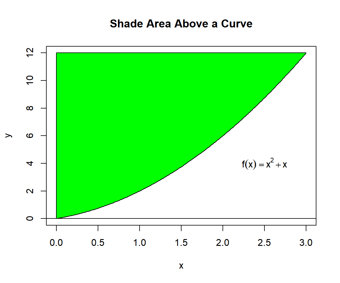
Shade Area Above a Curve in R
Region Above a Curve
Next, shaded regions above a curve using the function \(y=x^3\) as an example.
Shade regions: \(-0.9\leq x \leq -0.4\) with \(y \leq 0\), and \(0 \leq x \leq 0.5\) up to \(y = 1\).
To shade the blue region above the curve, start at the left top point (-0.9, 0), down to (-0.9, y = \(-0.9^3\)), follow the curve, all (x, y)’s for \(-0.9\leq x \leq -0.4\), up to (-0.4, y = \(-0.4^3\)), draw up to (-0.4, 0), then the function draws back to (-0.9, 0) and shades enclosed area.
To shade the red region above the curve, start at the left top point (0, 1), down to (0, 0), follow the curve, all (x, y)’s for \(0 \leq x \leq 0.5\), up to (0.5, y = \(0.5^3\)), draw up to (0.5, 1), then the function draws back to (0, 1) and shades enclosed area.
x = seq(-1, 1, 1/100); y = x^(3)
plot(x, y, type = "l",
     main = "Shade Regions Above a Curve")
abline(h = 0)
text(0.8, 0.25, expression(f(x) == x^3))

# Blue area: specify the x and y points in enclosing order.
polygon(x = c(-0.9, -0.9, x[x > -0.9 & x < -0.4], -0.4, -0.4),
        y = c(0, (-0.9)^3, y[x > -0.9 & x < -0.4], (-0.4)^3, 0),
        col = "blue")

# Red area: specify the x and y points in enclosing order.
polygon(x = c(0, 0, x[x>0 & x<0.5], 0.5, 0.5),
        y = c(1, 0, y[x>0 & x<0.5], 0.5^3, 1),
        col = "red")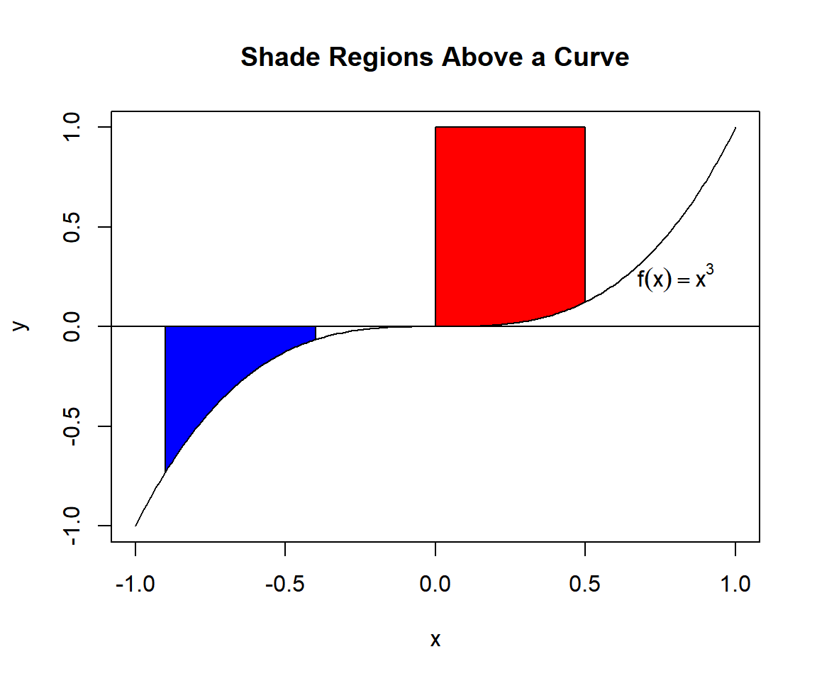
Shade Regions Above a Curve in R
4 Shade Area & Region Between Two Curves in R
Here we show how to shade the area between two curves using the
polygon() function.
Using the functions \(y=x^2\) and \(y=\sqrt{2x}\) as an example.
Shade areas: between the two solutions of \(x\) and beyond the second solution of \(x\).
To shade the green area between the two curves, follow the upper curve, all (x, y)’s between the two solutions (\(0\leq x \leq 1.259921\)), then follow the lower curve in reverse with
rev(), between the two solutions, then the function shades enclosed area.To shade the pink region between the two curves, follow the upper curve, all (x, y)’s between the second solution and end point (\(1.259921\leq x \leq 2\)), then follow the lower curve in reverse with
rev(), between the second solution and end point, then the function shades enclosed area.
x = seq(0, 2, 1/100); y1 = x^(2); y2 = sqrt(2*x)
plot(x, y1, type = "l",
     main = "Shade Area & Region Between Two Curves")
points(x, y2, type = "l")
text(1.5, 3, expression(f(x) == x^2))
text(1.75, 1, expression(f(x) == sqrt(2*x)))

# Green area: specify the x and y points in enclosing order.
sol1 = 0        # first solution
sol2 = 1.259921 # second solution
polygon(x = c(x[x>=sol1 & x<=sol2], rev(x[x>=sol1 & x<=sol2])),
        y = c(y1[x>=sol1 & x<=sol2], rev(y2[x>=sol1 & x<=sol2])),
        col = "green")

# Pink area: specify the x and y points in enclosing order.
sol = 1.259921
end = 2
polygon(x = c(x[x>=sol & x<=end], rev(x[x>=sol & x<=end])),
        y = c(y1[x>=sol & x<=end], rev(y2[x>=sol & x<=end])),
        col = "pink")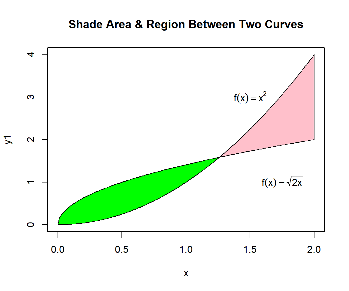
Shade Area & Region Between Two Curves in R
The feedback form is a Google form but it does not collect any personal information.
Please click on the link below to go to the Google form.
Thank You!
Go to Feedback Form
Copyright © 2020 - 2026. All Rights Reserved by Stats Codes