1 Plotting Simple Functions in R
2 Plotting Multiple Curved Functions in One Plot with Equations or Legend in R
3 Set Title, Labels, Limits, Colors, Line Type & Width, Points, Fonts of a Plotted Function in R
4 Plot a Function with Dots in R

Here, we show how to plot single or multiple functions in R: including linear and curved functions and setting line widths and colors.

These are done with the curve() and plot() functions. The curve() function takes both expressions and R functions as argument while the plot() function takes only R functions as argument.

See plots & charts for graphical parameters and other plots and charts.

1 Plotting Simple Functions in R

To plot a simple function, for example, \[y = 2x^2 - x + 5,\] from \(-2\) to \(5\). Use the curve() function as follows:

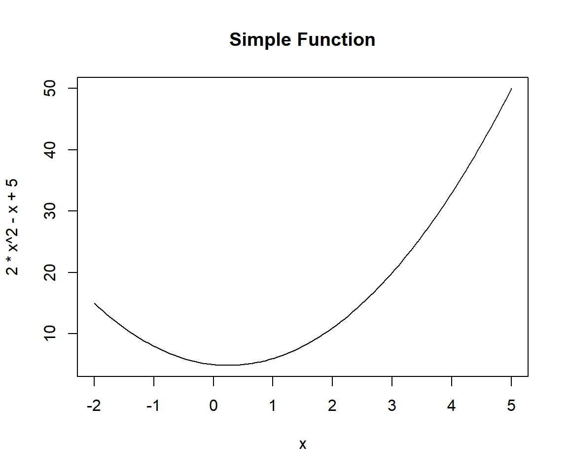
curve(2*x^2 - x + 5, -2, 5, main = "Simple Function")

Example 1: Plotting a Simple Curved Function in R

Or by calling the equation:

equation = function(x){2*x^2 - x + 5}
curve(equation, -2, 5, main = "Simple Function")
plot(equation, -2, 5, main = "Simple Function")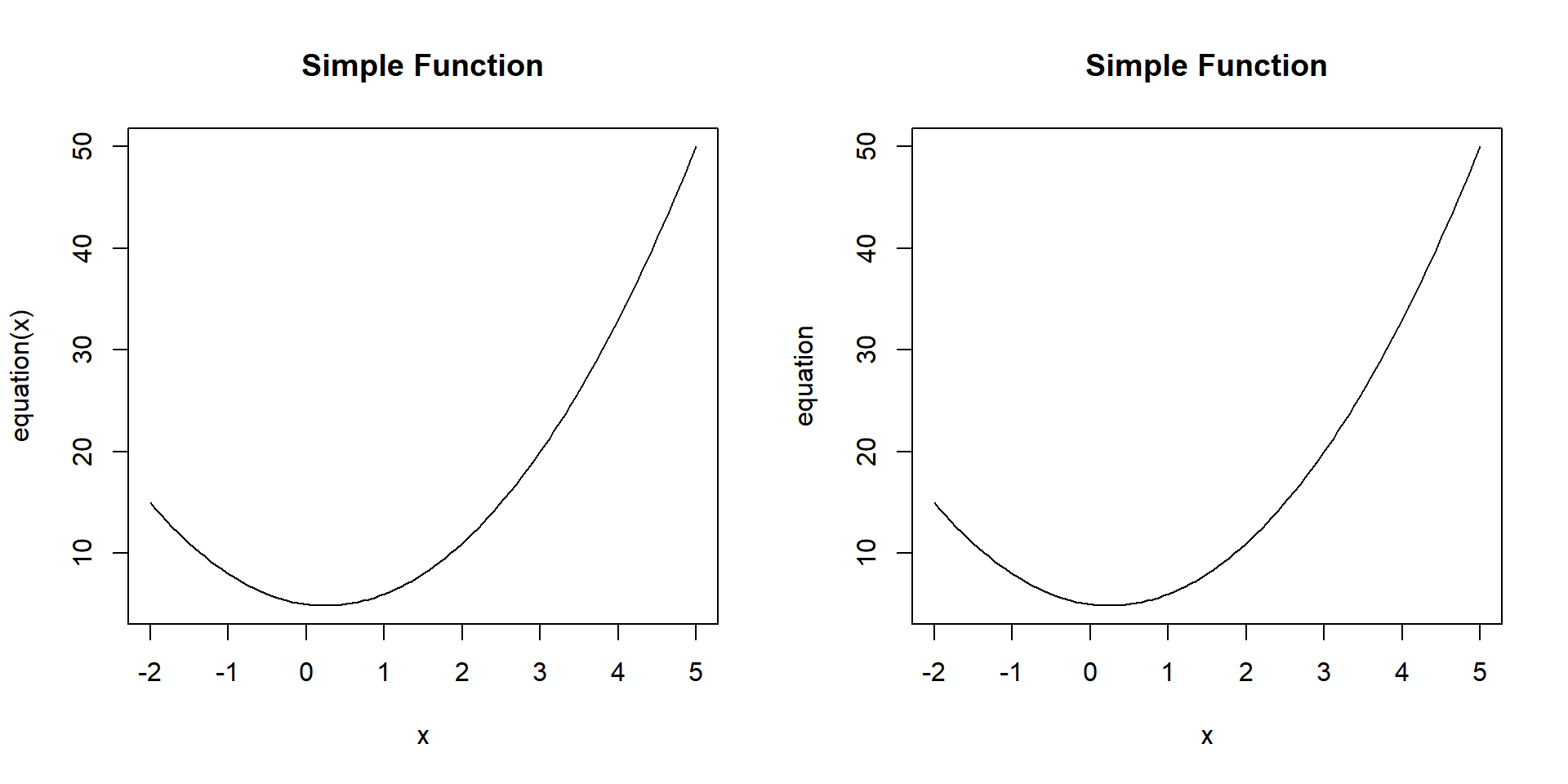

Example 2: Plotting a Simple Curved Function in R

2 Plotting Multiple Curved Functions in One Plot with Equations or Legend in R

With Equations on Plot:

You can plot both \(x^3 - 2x\) and \(4x\) from \(-3\) to \(3\) with equations and expressions on the plot as follows.

curve(x^3 - 2*x, -3, 3, col = "blue",
      ylab = "f(x)",
      main = expression(paste("Plots of ", x^3 - 2*x, " and ", 4*x)))
text(2.5, 0, expression(f(x) == x^3 - 2*x), col = "blue")

curve(4*x, -3, 3, add  = TRUE, col = "red", lty = 3, lwd = 2)
text(-1.5, -10, expression(f(x) == 4*x), col = "red")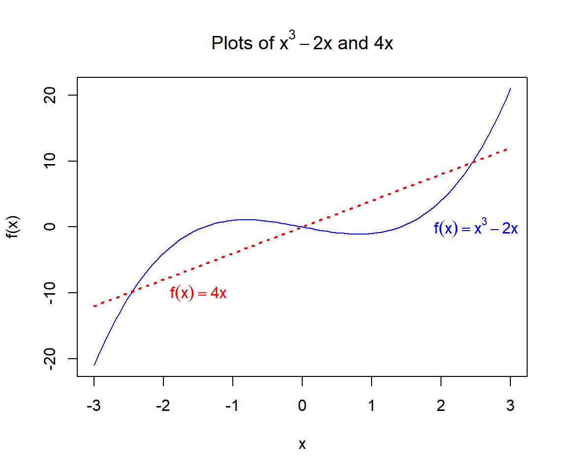

Plotting Multiple Curved Functions in One Plot - with Equations - in R

With Legend on Plot:

You can plot both the \(sin\) and \(cos\) functions from \(-2\pi\) to \(2\pi\) with a legend as follows.

curve(sin, -2*pi, 2*pi, col = "blue", lwd = 3,
      ylab = "sin(x) & cos(x)",
      main = "Trigonometric Functions")
curve(cos, -2*pi, 2*pi, add  = TRUE, col = "red", lty = 4, lwd = 1.5)

legend("topright", c("sin(x)", "cos(x)"), fill = c("blue", "red"))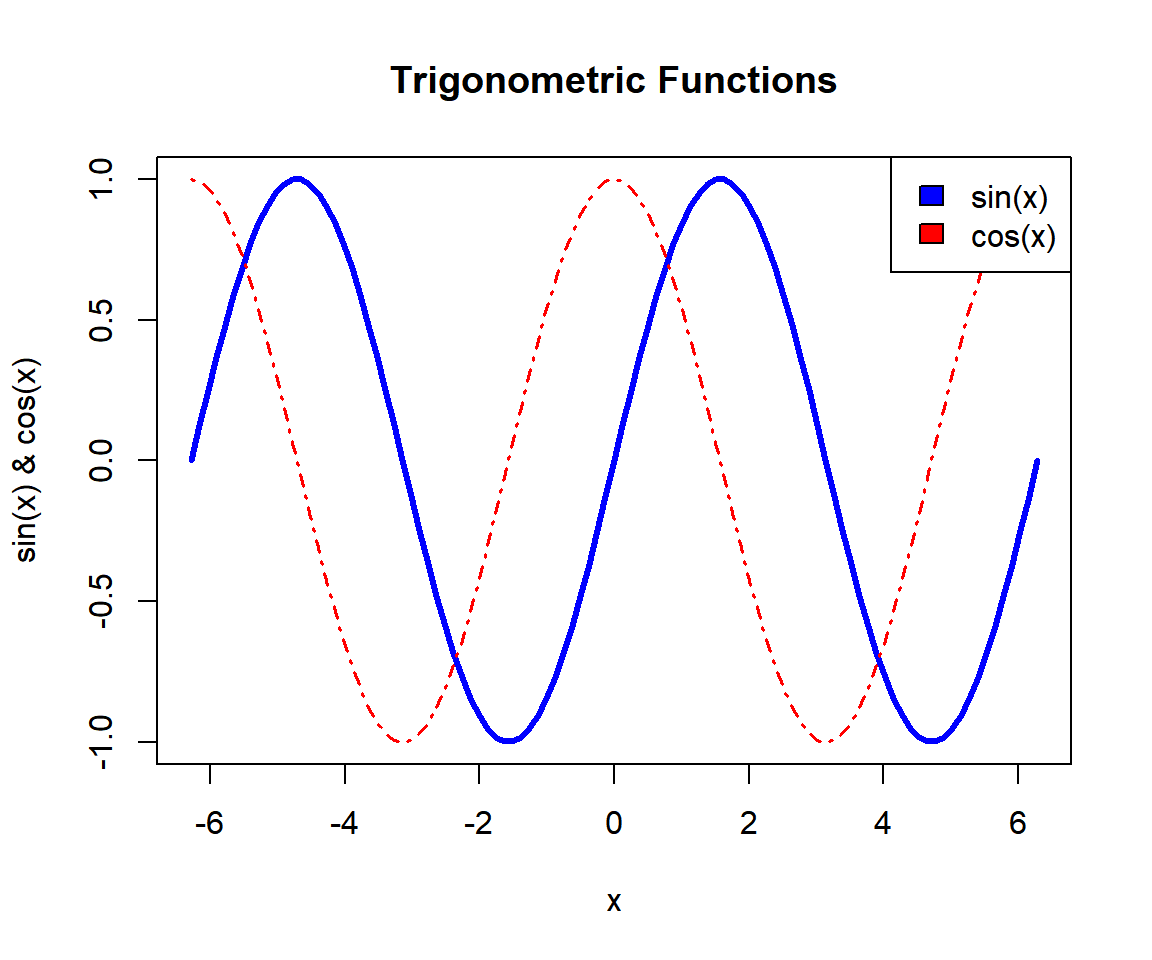

Plotting Multiple Curved Functions in One Plot - with Legend - in R

3 Set Title, Labels, Limits, Colors, Line Type & Width, Points, Fonts of a Plotted Function in R

Here we set details such as title (main), x-axis and y-axis labels (xlab, ylab), limits (xlim, ylim), colors (col), line type (lty) & width (lwd), font types (font), and font sizes (cex). See also setting colors and fonts for more details.

curve(x^3, main = expression(paste("Plots of ", x^3)),
      xlab = "X Value", ylab = "Y Value",
      xlim = c(-2, 2),  ylim = c(-8, 8),
      col = "blue",
      col.main="blue", col.lab="red", col.axis="tan",
      lty = 3, lwd = 2.5,
      font=4, font.lab=4, font.main=2,
      cex.main=1.5, cex.lab=1.2, cex.axis=1)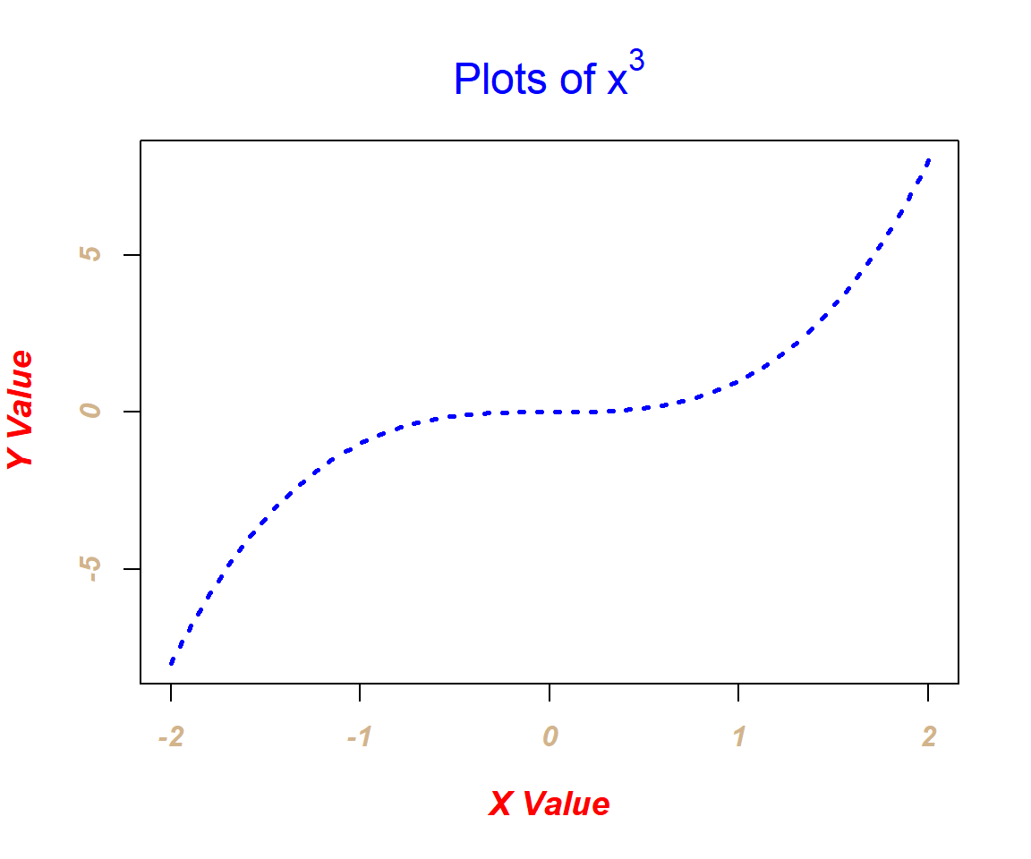

Plotted Function with Title, Labels, Limits, Colors, Line Type & Width, and Fonts Set in R

4 Plot a Function with Dots in R

Here we plot a function with dots by setting the plot type (type), dot types (pch) and number of dots (n). See also point types and sizes for more details.

curve(x^2 - 2*x, main = "Plot with Dots",
      xlab = "x", ylab = "f(x)",
      xlim = c(-2, 2),  ylim = c(-3, 10),
      col = "red",
      col.main="green", col.lab="red", col.axis="blue",
      type = "p", pch = 5, n = 20,
      font=4, font.lab=4, font.main=2,
      cex.main=1.5, cex.lab=1.2, cex.axis=1)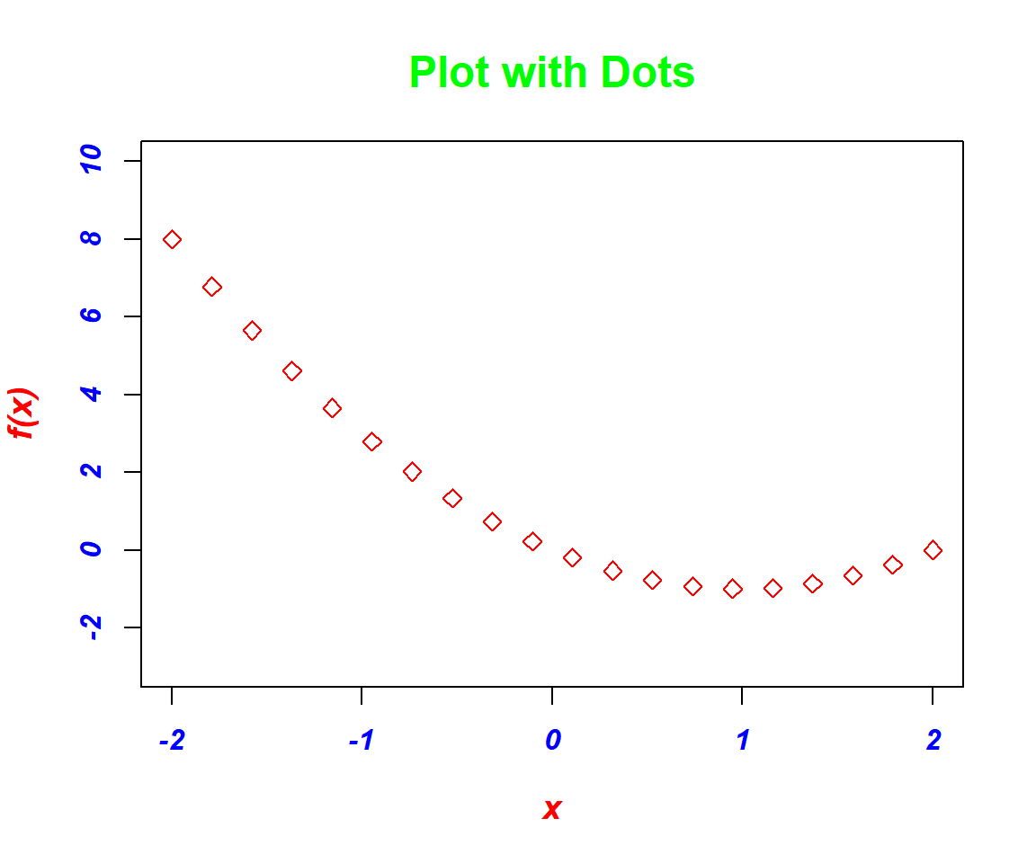

Plotted Function with Dots in R

Home About Terms