1 Table of Exponential Distribution Functions in R
2 Plot of Exponential Distributions in R
3 Examples for Setting Parameters for Exponential Distributions in R
4 rexp(): Random Sampling from Exponential Distributions in R
5 dexp(): Probability Density Function for Exponential Distributions in R
6 pexp(): Cumulative Distribution Function for Exponential Distributions in R
7 qexp(): Derive Quantile for Exponential Distributions in R

Here, we discuss exponential distribution functions in R, plots, parameter setting, random sampling, density, cumulative distribution and quantiles.

The exponential distribution with parameter \(\tt{rate}=\lambda\) has probability density function (pdf) formula as:

\[f(x) = \begin{cases} \lambda e^{ - \lambda x} & x \ge 0, \\ 0 & x < 0. \end{cases},\] where \(\lambda > 0\), and \(e\) is \(\tt{Euler's\;number}\) with \(e \approx 2.71828\).

The mean is \(\frac{1}{\lambda}\), and the variance is \(\frac{1}{\lambda^2}\).

1 Table of Exponential Distribution Functions in R

The table below shows the functions for exponential distributions in R.

Table of Exponential Distribution Functions in R
Function	Usage
rexp(n, rate = 1)	Simulate a random sample with \(n\) observations
dexp(x, rate = 1)	Calculate the probability density at the point \(x\)
pexp(q, rate = 1)	Calculate the cumulative distribution at the point \(q\)
qexp(p, rate = 1)	Calculate the quantile value associated with \(p\)

2 Plot of Exponential Distributions in R

Single distribution:

Below is a plot of the exponential distribution function with \(\tt{rate}=0.2\).

x = seq(0, 35, 1/1000); y = dexp(x, 0.2)
plot(x, y, type = "l",
     xlim = c(0, 35), ylim = c(0, max(y)),
     main = "Probability Density Function of
Exponential Distribution (0.2)",
     xlab = "x",  ylab = "Density",
     lwd = 2, col = "blue")
# Add legend
legend("topright", "rate = 0.2",
       lwd = 2,
       col = "blue",
       bty = "n")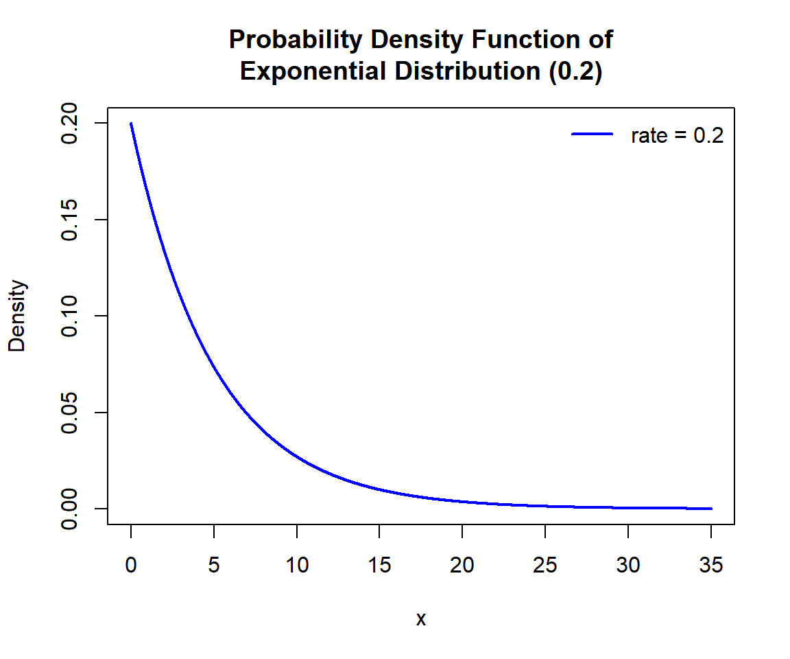

Probability Density Function (PDF) of an Exponential Distribution in R

Multiple distributions:

Below is a plot of multiple exponential distribution functions in one graph.

x1 = seq(0, 10, 1/1000); y1 = dexp(x1, 2)
x2 = seq(0, 10, 1/1000); y2 = dexp(x2, 1)
x3 = seq(0, 10, 1/1000); y3 = dexp(x3, 0.5)
plot(x1, y1, type = "l",
     xlim = c(0, 10), ylim = range(c(y1, y2, y3)),
     main = "Probability Density Functions of Exponential Distributions",
     xlab = "x", ylab = "Density",
     lwd = 2, col = "blue")
points(x2, y2, type = "l", lwd = 2, col = "red")
points(x3, y3, type = "l", lwd = 2, col = "green")
# Add legend
legend("topright", c("rate = 2",
                    "rate = 1",
                    "rate = 0.5"),
       lwd = c(2, 2, 2),
       col = c("blue", "red", "green"),
       bty = "n")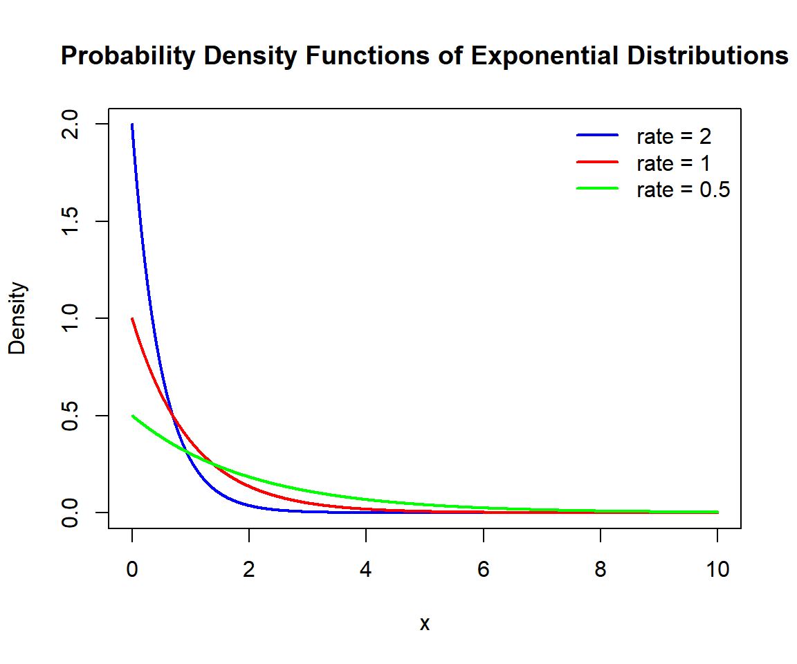

Probability Density Functions (PDFs) of Exponential Distributions in R

3 Examples for Setting Parameters for Exponential Distributions in R

In the exponential distribution functions, the rate parameter is pre-specified as \(\tt{rate}=1\), hence it does not need to be specified, unless it is to be set to a different value.

For example, for qexp(), the following are the same:

qexp(0.2); qexp(0.2, 1)

[1] 0.2231436

[1] 0.2231436

qexp(0.2, rate = 1)

[1] 0.2231436

4 rexp(): Random Sampling from Exponential Distributions in R

Sample 1200 observations from the exponential distribution with \(\tt{rate}=2\):

rexp(1200, 2)

set.seed(500) # Line allows replication (use any number).
sample = rexp(1200, 2)
hist(sample,
     main = "Histogram of 1200 Observations from 
Exponential Distribution with Rate = 2",
     xlab = "x",
     col = "deepskyblue", border = "white")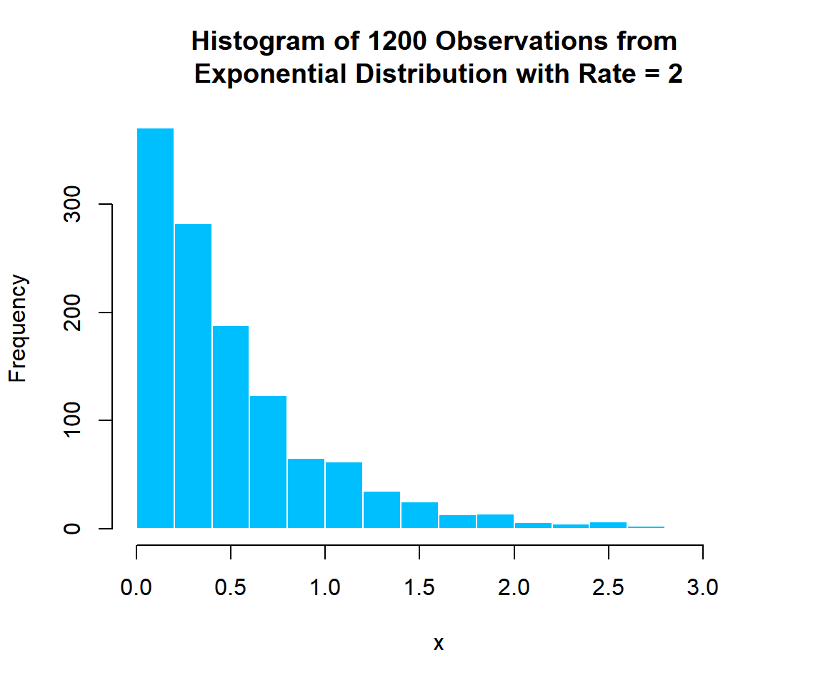

Histogram of Exponential Distribution (2) Random Sample in R

5 dexp(): Probability Density Function for Exponential Distributions in R

Calculate the density at \(x = 0.5\), in the exponential distribution with \(\tt{rate} = 3\):

dexp(0.5, 3)

[1] 0.6693905

x = seq(0, 3, 1/1000); y = dexp(x, 3)
plot(x, y, type = "l",
     xlim = c(0, 3), ylim = c(0, max(y)),
     main = "Probability Density Function of Exponential Distribution
with Rate = 3",
     xlab = "x", ylab = "Density",
     lwd = 2, col = "blue")
# Add lines
segments(0.5, -1, 0.5, 0.6693905)
segments(-1, 0.6693905, 0.5, 0.6693905)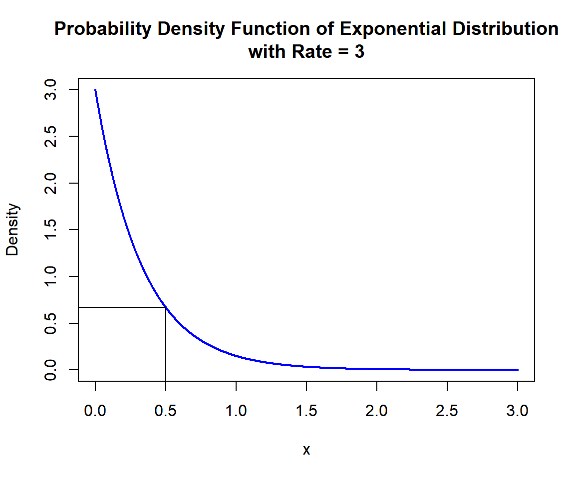

Probability Density Function (PDF) of Exponential Distribution (3) in R

6 pexp(): Cumulative Distribution Function for Exponential Distributions in R

Calculate the cumulative distribution at \(x = 2.3\), in the exponential distribution with \(\tt{rate} = 0.6\). That is, \(P(X \le 2.3)\):

pexp(2.3, 0.6)

[1] 0.7484214

x = seq(0, 10, 1/1000); y = pexp(x, 0.6)
plot(x, y, type = "l",
     xlim = c(0, 10), ylim = c(0,1),
     main = "Cumulative Distribution Function of
Exponential Distribution with Rate = 0.6",
     xlab = "x", ylab = "Cumulative Distribution",
     lwd = 2, col = "blue")
# Add lines
segments(2.3, -1, 2.3, 0.7484214)
segments(-1, 0.7484214, 2.3, 0.7484214)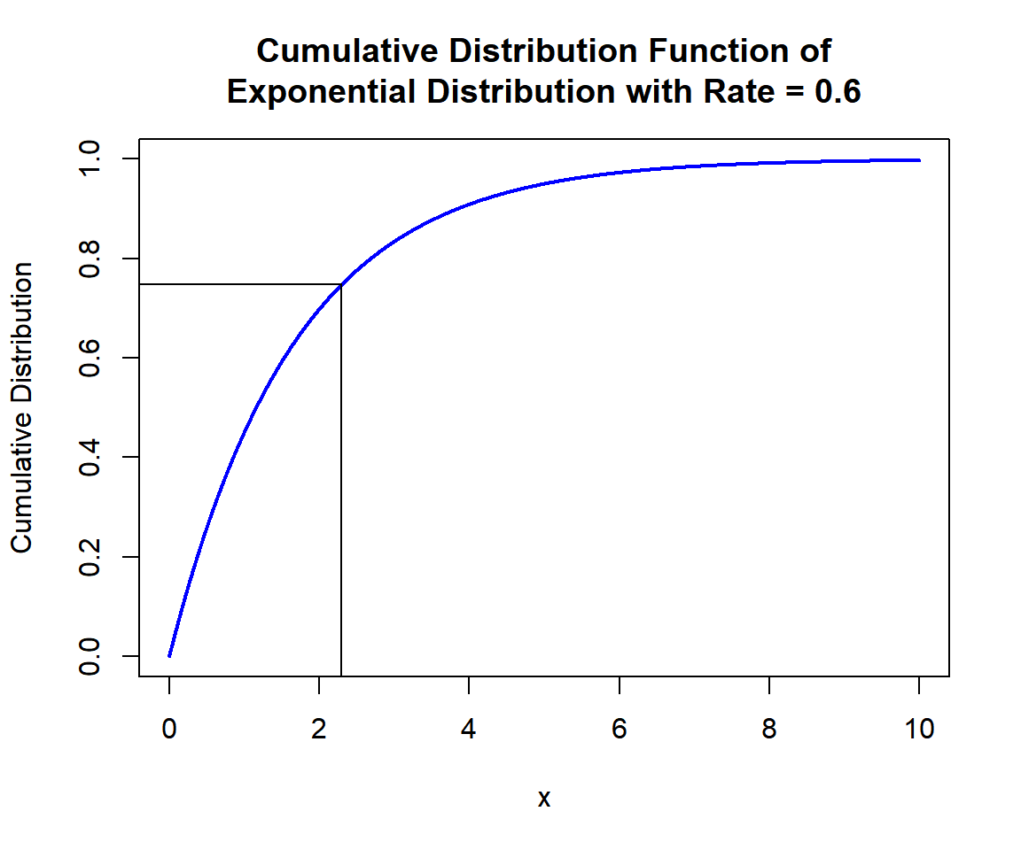

Cumulative Distribution Function (CDF) of Exponential Distribution (0.6) in R

x = seq(0, 10, 1/1000); y = dexp(x, 0.6)
plot(x, y, type = "l",
     xlim = c(0, 10), ylim = c(0, max(y)),
     main = "Probability Density Function of Exponential Distribution
with Rate = 0.6",
     xlab = "x", ylab = "Density",
     lwd = 2, col = "blue")
# Add shaded region and legend
point = 2.3
polygon(x = c(0, x[x <= point], point),
        y = c(0, y[x <= point], 0),
        col = "limegreen")
legend("topright", c("Area = 0.7484214"),
       fill = c("limegreen"),
       inset = 0.01)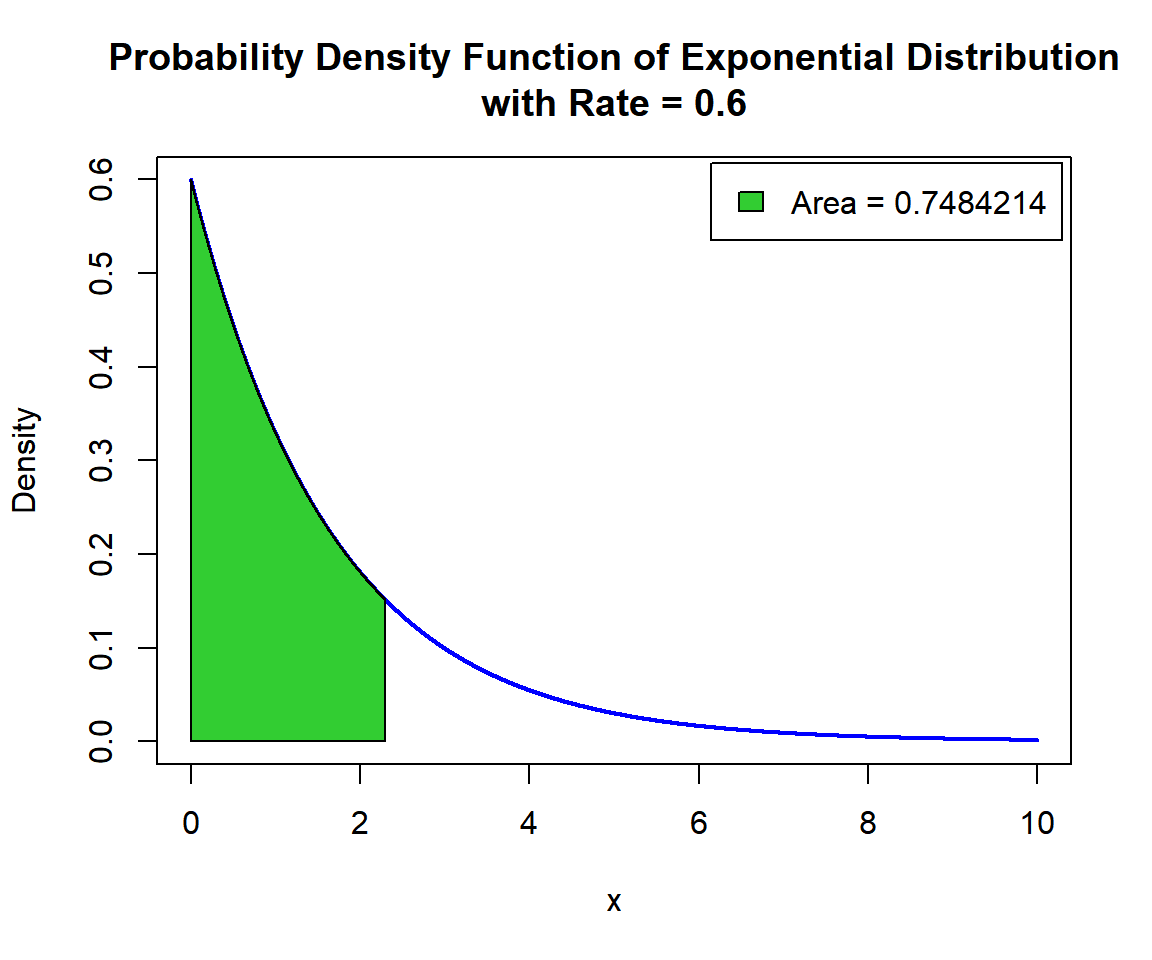

Shaded Probability Density Function (PDF) of Exponential Distribution (0.6) in R

For upper tail, at \(x = 2.3\), that is, \(P(X \ge 2.3) = 1 - P(X \le 2.3)\), set the "lower.tail" argument:

pexp(2.3, 0.6, lower.tail = FALSE)

[1] 0.2515786

x = seq(0, 10, 1/1000); y = dexp(x, 0.6)
plot(x, y, type = "l",
     xlim = c(0, 10), ylim = c(0, max(y)),
     main = "Shaded Upper Region: Probability Density Function
of Exponential Distribution with Rate = 0.6",
     xlab = "x", ylab = "Density",
     lwd = 2, col = "blue")
# Add shaded region and legend
point = 2.3
polygon(x = c(point, x[x >= point]),
        y = c(0, y[x >= point]),
        col = "limegreen")
legend("topright", c("Area = 0.2515786"),
       fill = c("limegreen"),
       inset = 0.01)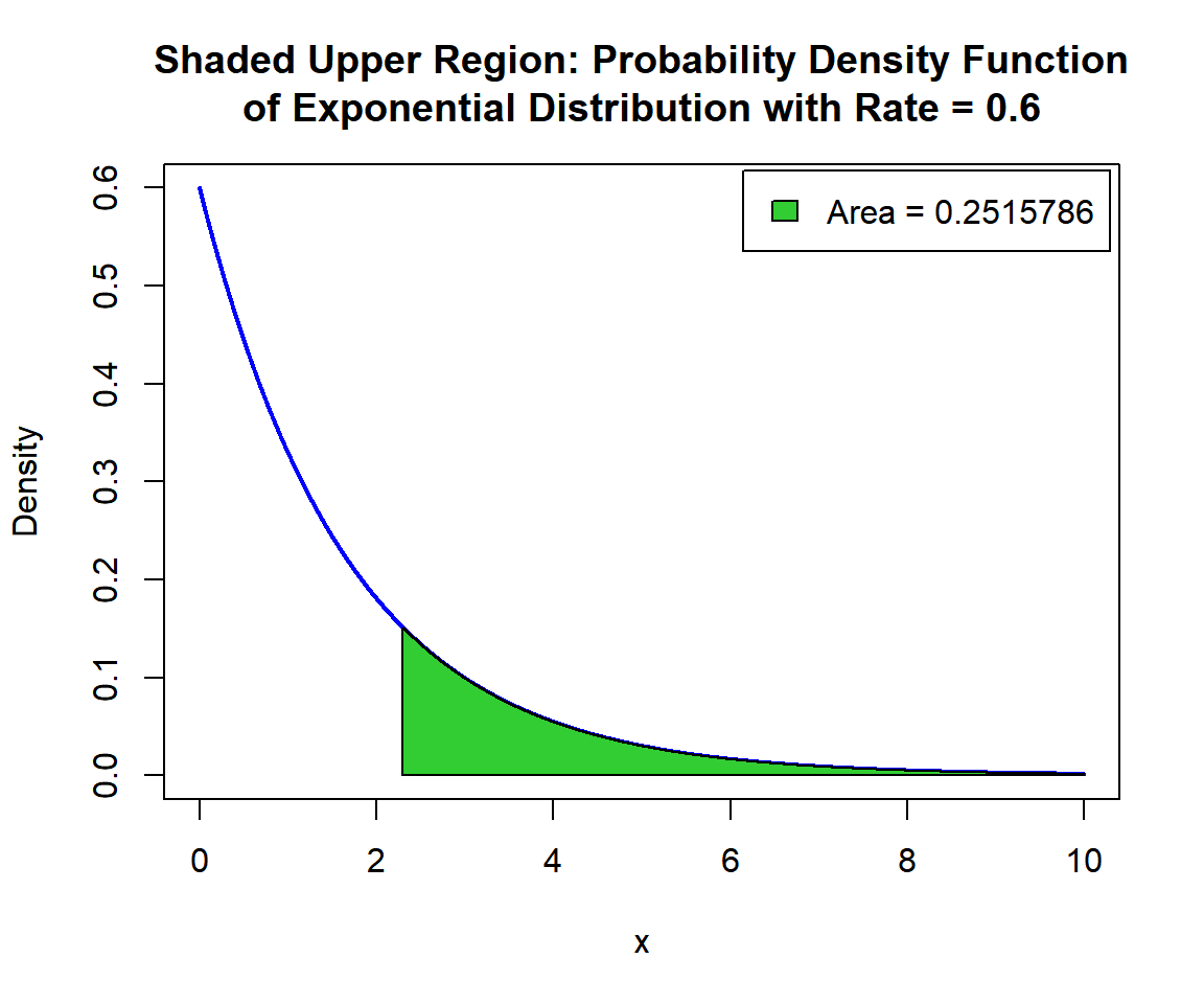

Shaded Upper Region: Probability Density Function (PDF) of Exponential Distribution (0.6) in R

7 qexp(): Derive Quantile for Exponential Distributions in R

Derive the quantile for \(p = 0.85\), in the exponential distribution with \(\tt{rate} = 0.8\). That is, \(x\) such that, \(P(X \le x)=0.85\):

qexp(0.85, 0.8)

[1] 2.3714

x = seq(0, 7, 1/1000); y = pexp(x, 0.8)
plot(x, y, type = "l",
     xlim = c(0, 7), ylim = c(0,1),
     main = "Cumulative Distribution Function of
Exponential Distribution with Rate = 0.8",
     xlab = "x", ylab = "Cumulative Distribution",
     lwd = 2, col = "blue")
# Add lines
segments(2.3714, -1, 2.3714, 0.85)
segments(-1, 0.85, 2.3714, 0.85)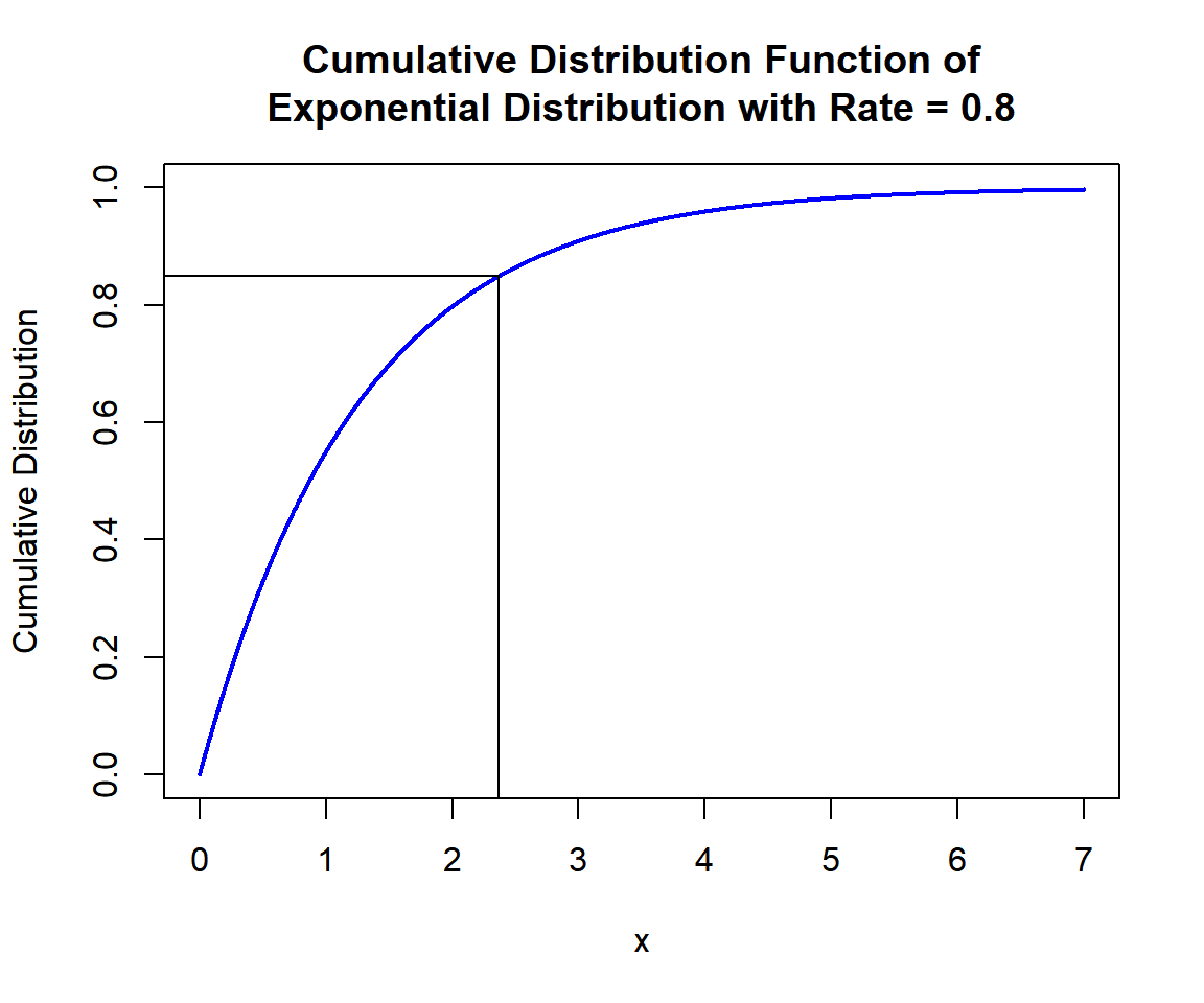

Cumulative Distribution Function (CDF) of Exponential Distribution (0.8) in R

x = seq(0, 7, 1/1000); y = dexp(x, 0.8)
plot(x, y, type = "l",
     xlim = c(0, 7), ylim = c(0, max(y)),
     main = "Probability Density Function of Exponential Distribution
with Rate = 0.8",
     xlab = "x", ylab = "Density",
     lwd = 2, col = "blue")
# Add shaded region and legend
point = 2.3714
polygon(x = c(0, x[x <= point], point),
        y = c(0, y[x <= point], 0),
        col = "limegreen")
legend("topright", c("Area = 0.85"),
       fill = c("limegreen"),
       inset = 0.01)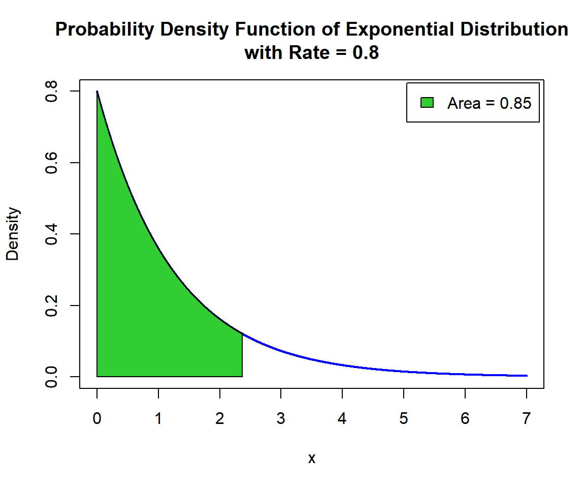

Shaded Probability Density Function (PDF) of Exponential Distribution (0.8) in R

For upper tail, for \(p = 0.15\), that is, \(x\) such that, \(P(X \ge x)=0.15\):

qexp(0.15, 0.8, lower.tail = FALSE)

[1] 2.3714

x = seq(0, 7, 1/1000); y = dexp(x, 0.8)
plot(x, y, type = "l",
     xlim = c(0, 7), ylim = c(0, max(y)),
     main = "Shaded Upper Region: Probability Density Function
of Exponential Distribution with Rate = 0.8",
     xlab = "x", ylab = "Density",
     lwd = 2, col = "blue")
# Add shaded region and legend
point = 2.3714
polygon(x = c(point, x[x >= point]),
        y = c(0, y[x >= point]),
        col = "limegreen")
legend("topright", c("Area = 0.15"),
       fill = c("limegreen"),
       inset = 0.01)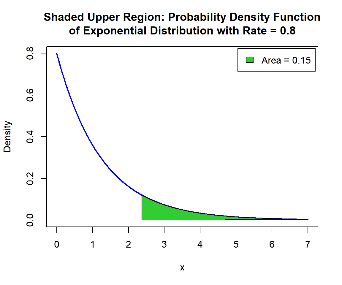

Shaded Upper Region: Probability Density Function (PDF) of Exponential Distribution (0.8) in R