Paired Two Sample T-tests (Matched Pairs) in R
- 1 Test Statistic for Paired Two Sample T-test in R
- 2 Simple Paired Two Sample T-test in R
- 3 Paired Two Sample T-test Critical Value in R
- 4 Two-tailed Paired Two Sample T-test in R
- 5 One-tailed Paired Two Sample T-test in R
- 6 Paired Two Sample T-test: Test Statistics, P-value & Degree of Freedom in R
- 7 Paired Two Sample T-test: Estimates, Standard Error & Confidence Interval in R
Here, we discuss the paired two sample t-test in R with interpretations, including, test statistics, p-values, critical values, confidence intervals, and standard errors.
The paired two sample t-test in R can be performed with the
t.test() function from the base "stats" package.
The paired two sample t-test is also the dependent two sample t-test. It can be used to test whether the mean of the differences between matched pairs in the population of matched pairs where an independent random sample of matched pairs comes from is equal to a certain value (which is stated in the null hypothesis) or not.
In the paired two sample t-test, the test statistic follows a Student’s t-distribution when the null hypothesis is true.
| Question | Is the mean of paired x and y differences equal \(d_0\)? | Is the mean of paired x and y differences greater than \(d_0\)? | Is the mean of paired x and y differences less than \(d_0\)? |
| Form of Test | Two-tailed | Right-tailed test | Left-tailed test |
| Null Hypothesis, \(H_0\) | \(\mu_d = d_0\) | \(\mu_d = d_0\) | \(\mu_d = d_0\) |
| Alternate Hypothesis, \(H_1\) | \(\mu_d \neq d_0\) | \(\mu_d > d_0\) | \(\mu_d < d_0\) |
Sample Steps to Run a Paired Two Sample T-test:
# Create the data samples for the paired two Sample t-test
# Values are paired based on matching position in each sample

data_x = c(7.9, 9.3, 9.0, 7.1, 9.9)
data_y = c(7.6, 5.0, 8.9, 12.8, 8.3)

# Run the paired two sample t-test with specifications

t.test(data_x, data_y, paired = TRUE,
       alternative = "two.sided",
       mu = 0, conf.level = 0.95)
# Or
t.test(Pair(data_x, data_y) ~ 1,
       alternative = "two.sided",
       mu = 0, conf.level = 0.95)
    Paired t-test

data:  data_x and data_y
t = -0.049991, df = 5, p-value = 0.9621
alternative hypothesis: true mean difference is not equal to 0
95 percent confidence interval:
 -3.494752  3.361418
sample estimates:
mean difference
-0.06666667 | Argument | Usage |
| x, y | The two sample data values |
| paired | Set to TRUE for paired two sample t-test |
| Pair(x, y) ~ 1 | Can be used in place of "paired = TRUE" |
| alternative | Set alternate hypothesis as "greater", "less", or the default "two.sided" |
| mu | The population mean of difference between paired values in the null hypothesis |
| conf.level | Level of confidence for the test and confidence interval (default = 0.95) |
Creating a Paired Two Sample T-test Object:
# Create data
data_x = rnorm(200); data_y = rnorm(200)

# Create object
test_object = t.test(data_x, data_y, paired = TRUE,
                     alternative = "two.sided",
                     mu = 0, conf.level = 0.95)

# Extract a component
test_object$statistic
t
-0.515565 | Test Component | Usage |
| test_object$statistic | t-statistic value |
| test_object$p.value | P-value |
| test_object$parameter | Degrees of freedom |
| test_object$estimate | Point estimate or sample mean differences |
| test_object$stderr | Standard error value |
| test_object$conf.int | Confidence interval |
1 Test Statistic for Paired Two Sample T-test in R
The paired two sample t-test has test statistics, \(t\), of the form:
\[t = \frac{\bar d - d_0}{s_d/ \sqrt{n}} = \frac{(\bar x - \bar y) - d_0}{s_d/ \sqrt{n}}.\] For an independent random sample of matched pairs’ differences that comes from a normal distributions or for large sample sizes (for example, pairs of \(n > 30\)), \(t\) is said to follow the Student’s t-distribution when the null hypothesis is true, with the degrees of freedom as \(n-1\).
With \(d = x - y\), as the paired differences,
\(\bar d\) is the sample mean of the paired differences,
\(\bar x\) and \(\bar y\) are the sample means,
\(d_0\) is the population mean of paired differences to be tested and set in the null hypothesis,
\(s_d\) is the sample standard deviation of the paired differences, and
\(n\) is the sample size or number of pairs.
See also one sample t-tests and two sample t-tests (independent & unequal variance and independent & equal variance).
For non-parametric tests, see the sign test for paired samples and the Wilcoxon signed-rank test for paired samples.
2 Simple Paired Two Sample T-test in R
Enter the data by hand.
data_x = c(120.7, 115.8, 132.5, 114.5, 115.0,
          129.7, 119.4, 125.2, 127.8, 118.0,
          122.8, 121.6, 120.3, 110.8, 106.1)
data_y = c(103.4, 115.5, 129.4, 115.2, 123.4,
          113.8, 117.3, 131.2, 121.9, 114.9,
          134.3, 125.2, 122.6, 115.5, 115.5)
For data_x as the \(x\) group and data_y as the \(y\) group.
The sample means are \(\bar x =
120.0133333\) (mean(data_x)), and \(\bar y = 119.94\)
(mean(data_y)).
For the following null hypothesis \(H_0\), and alternative hypothesis \(H_1\), with the level of significance \(\alpha=0.05\).
\(H_0:\) population mean of the paired differences is equal to 0 (\(\mu_d = 0\)).
\(H_1:\) population mean of the paired differences is not equal to 0 (\(\mu_d \neq 0\), hence the default two-sided).
Because the level of significance is \(\alpha=0.05\), the level of confidence is \(1 - \alpha = 0.95\).
The t.test() function has the default
alternative as "two.sided", the default mean of
differences as 0, and the default level of confidence
as 0.95, hence, you do not need to specify the "alternative",
"mu", and "conf.level" arguments in this case.
Or:
    Paired t-test

data:  data_x and data_y
t = 0.033972, df = 14, p-value = 0.9734
alternative hypothesis: true mean difference is not equal to 0
95 percent confidence interval:
 -4.556505  4.703172
sample estimates:
mean difference
     0.07333333
The sample mean of the paired differences, \(\bar d\), is 0.07333333 ,
test statistic, \(t\), is 0.033972,
the degrees of freedom, \(n-1\), is 14,
the p-value, \(p\), is 0.9734,
the 95% confidence interval is [-4.556505 4.703172].
Interpretation:
P-value: With the p-value (\(p = 0.9734\)) being greater than the level of significance 0.05, we fail to reject the null hypothesis that the population mean of the paired differences is equal to 0.
\(t\)-statistic: With test statistics value (\(t = 0.033972\)) being between the two critical values, \(-t_{n-1,\alpha/2}=\text{qt(0.025, 14)}=-2.1447867\) and \(t_{n-1,\alpha/2}=\text{qt(0.975, 14)}=2.1447867\) (or not in the shaded region), we fail to reject the null hypothesis that the population mean of the paired differences is equal to 0.
Confidence Interval: With the null hypothesis population mean of the paired differences value (\(\mu_d = 0\)) being inside the confidence interval, \([-4.556505, 4.703172]\), we fail to reject the null hypothesis that population mean of the paired differences is equal to 0.
x = seq(-4, 4, 1/1000); y = dt(x, df=14)
plot(x, y, type = "l",
     xlim = c(-4, 4), ylim = c(-0.03, max(y)),
     main = "Paired Two Sample Student's T-test
Shaded Region for Simple T-test",
     xlab = "x", ylab = "Density",
     lwd = 2, col = "blue")
abline(h=0)
# Add shaded region and legend
point1 = qt(0.025, 14); point2 = qt(0.975, 14)
polygon(x = c(-4, x[x <= point1], point1),
        y = c(0, y[x <= point1], 0),
        col = "blue")
polygon(x = c(x[x >= point2], 4, point2),
        y = c(y[x >= point2], 0, 0),
        col = "blue")
legend("topright", c("Area = 0.05"),
       fill = c("blue"), inset = 0.01)
# Add critical value and t-value
arrows(0, 0.1, 0.033972, 0)
text(0, 0.12, "t = 0.033972")
text(-2.144787, -0.02, expression(-t[n-1][','][alpha/2]==-2.144787))
text(2.144787, -0.02, expression(t[n-1][','][alpha/2]==2.144787))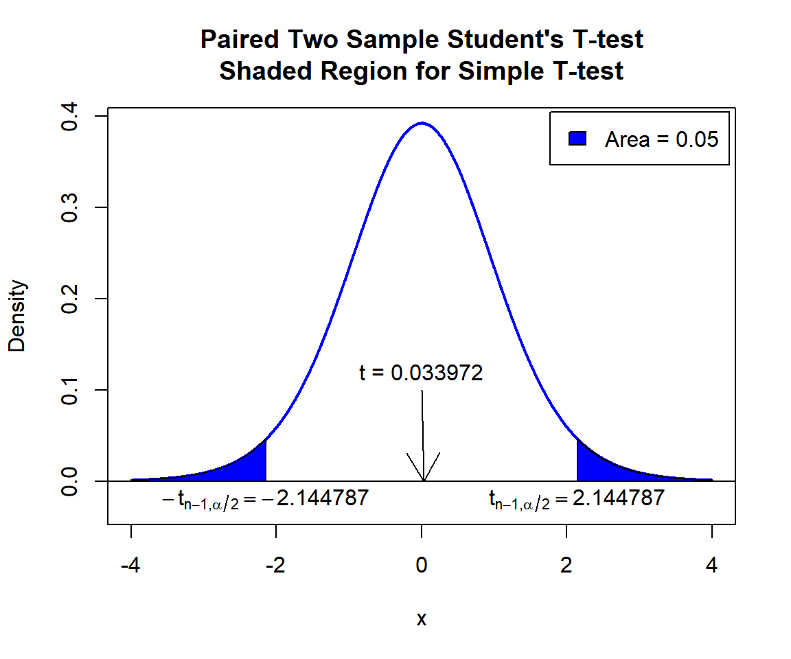
Paired Two Sample Student’s T-test Shaded Region for Simple T-test in R
See line charts, shading areas under a curve, lines & arrows on plots, mathematical expressions on plots, and legends on plots for more details on making the plot above.
3 Paired Two Sample T-test Critical Value in R
To get the critical value for a paired two sample t-test in R, you
can use the qt() function for Student’s t-distribution to
derive the quantile associated with the given level of significance
value \(\alpha\).
For two-tailed test with level of significance \(\alpha\). The critical values are: qt(\(\alpha/2\), df) and qt(\(1-\alpha/2\), df).
For one-tailed test with level of significance \(\alpha\). The critical value is: for left-tailed, qt(\(\alpha\), df); and for right-tailed, qt(\(1-\alpha\), df).
Example:
For \(\alpha = 0.05\), and \(\text{df = 19}\).
Two-tailed:
[1] -2.093024[1] 2.093024One-tailed:
[1] -1.729133[1] 1.7291334 Two-tailed Paired Two Sample T-test in R
Using the "Setosa" specie in the iris data (first 50 rows only) from the "datasets" package with 10 sample rows from 50 rows below:
   Sepal.Length Sepal.Width Petal.Length Petal.Width Species
1           5.1         3.5          1.4         0.2  setosa
5           5.0         3.6          1.4         0.2  setosa
19          5.7         3.8          1.7         0.3  setosa
23          4.6         3.6          1.0         0.2  setosa
25          4.8         3.4          1.9         0.2  setosa
30          4.7         3.2          1.6         0.2  setosa
36          5.0         3.2          1.2         0.2  setosa
44          5.0         3.5          1.6         0.6  setosa
49          5.3         3.7          1.5         0.2  setosa
50          5.0         3.3          1.4         0.2  setosa
For Sepal.Length as the \(x\) group versus Sepal.Width as the \(y\) group.
The sample means are \(\bar x =
5.006\) (mean(iris_data$Sepal.Length)), and \(\bar y = 3.428\)
(mean(iris_data$Sepal.Width)).
For the following null hypothesis \(H_0\), and alternative hypothesis \(H_1\), with the level of significance \(\alpha=0.1\).
\(H_0:\) population mean of the paired differences is equal to 1.5 (\(\mu_d = 1.5\)).
\(H_1:\) population mean of the paired differences is not equal to 1.5 (\(\mu_d \neq 1.5\), hence the default two-sided).
Because the level of significance is \(\alpha=0.1\), the level of confidence is \(1 - \alpha = 0.9\).
t.test(iris_data$Sepal.Length, iris_data$Sepal.Width,
       paired = TRUE,
       alternative = "two.sided",
       mu = 1.5, conf.level = 0.9)
    Paired t-test

data:  iris_data$Sepal.Length and iris_data$Sepal.Width
t = 2.092, df = 49, p-value = 0.04164
alternative hypothesis: true mean difference is not equal to 1.5
90 percent confidence interval:
 1.515491 1.640509
sample estimates:
mean difference
          1.578
Interpretation:
P-value: With the p-value (\(p = 0.04164\)) being lower than the level of significance 0.1, we reject the null hypothesis that the population mean of the paired differences is equal to 1.5.
\(t\)-statistic: With test statistics value (\(t = 2.092\)) being inside the critical region (shaded area), that is, \(t = 2.092\) greater than \(t_{n-1,\alpha/2}=\text{qt(0.95, 49)}=1.6765509\), we reject the null hypothesis that the population mean of the paired differences is equal to 1.5.
Confidence Interval: With the null hypothesis population mean of the paired differences value (\(\mu_d = 1.5\)) being outside the confidence interval, \([1.515491, 1.640509]\), we reject the null hypothesis that the population mean of the paired differences is equal to 1.5.
x = seq(-4, 4, 1/1000); y = dt(x, df=49)
plot(x, y, type = "l",
     xlim = c(-4, 4), ylim = c(-0.03, max(y)),
     main = "Paired Two Sample Student's T-test
Shaded Region for Two-tailed Test",
     xlab = "x", ylab = "Density",
     lwd = 2, col = "blue")
abline(h=0)
# Add shaded region and legend
point1 = qt(0.05, 49); point2 = qt(0.95, 49)
polygon(x = c(-4, x[x <= point1], point1),
        y = c(0, y[x <= point1], 0),
        col = "blue")
polygon(x = c(x[x >= point2], 4, point2),
        y = c(y[x >= point2], 0, 0),
        col = "blue")
legend("topright", c("Area = 0.1"),
       fill = c("blue"), inset = 0.01)
# Add critical value and t-value
arrows(2.092, 0.2, 2.092, 0)
text(2.092, 0.22, expression(t==2.092))
text(-1.676551, -0.02, expression(-t[n-1][','][alpha/2]==-1.676551))
text(1.676551, -0.02, expression(t[n-1][','][alpha/2]==1.676551))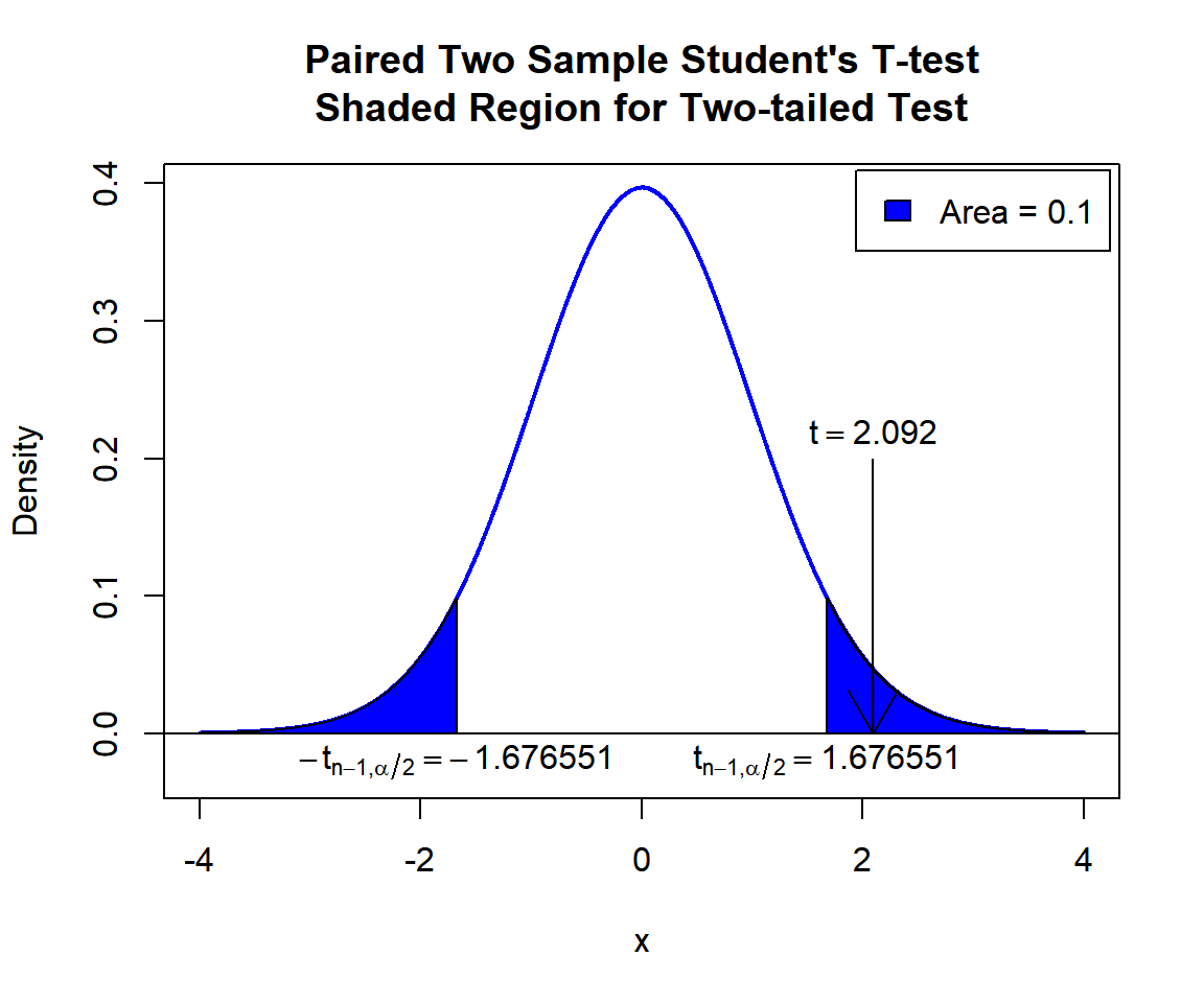
Paired Two Sample Student’s T-test Shaded Region for Two-tailed Test in R
5 One-tailed Paired Two Sample T-test in R
Right Tailed Test
Using the attitude data from the "datasets" package with 10 sample rows from 30 rows below:
   rating complaints privileges learning raises critical advance
1      43         51         30       39     61       92      45
7      58         67         42       56     66       68      35
11     64         53         53       58     58       67      34
13     69         62         57       42     55       63      25
15     77         77         54       72     79       77      46
17     74         85         64       69     79       79      63
20     50         58         68       54     64       78      52
24     40         37         42       58     50       57      49
27     78         75         58       74     80       78      49
30     82         82         39       59     64       78      39
For "critical" as the \(x\) group versus "raises" as the \(y\) group.
The sample means are \(\bar x =
74.7666667\) (mean(attitude$critical)), and \(\bar y = 64.6333333\)
(mean(attitude$raises)).
For the following null hypothesis \(H_0\), and alternative hypothesis \(H_1\), with the level of significance \(\alpha=0.15\).
\(H_0:\) population mean of the paired differences is equal to 5 (\(\mu_d = 5\)).
\(H_1:\) population mean of the paired differences is greater than 5 (\(\mu_d > 5\), hence one-sided).
Because the level of significance is \(\alpha=0.15\), the level of confidence is \(1 - \alpha = 0.85\).
t.test(attitude$critical, attitude$raises,
       paired = TRUE,
       alternative = "greater",
       mu = 5, conf.level = 0.85)
    Paired t-test

data:  attitude$critical and attitude$raises
t = 2.4807, df = 29, p-value = 0.00958
alternative hypothesis: true mean difference is greater than 5
85 percent confidence interval:
 7.94956     Inf
sample estimates:
mean difference
       10.13333
Interpretation:
P-value: With the p-value (\(p = 0.00958\)) being lower than the level of significance 0.15, we reject the null hypothesis that the population mean of the paired differences is equal to 5.
\(t\)-statistic: With test statistics value (\(t = 2.4807\)) being inside the critical region (shaded area), that is, \(t = 2.4807\) greater than \(t_{n-1,\alpha}=\text{qt(0.85, 29)}=1.0553022\), we reject the null hypothesis that the population mean of the paired differences is equal to 5.
Confidence Interval: With the null hypothesis population mean of the paired differences value (\(\mu_d = 5\)) being outside the confidence interval, \([7.94956, \infty)\), we reject the null hypothesis that the population mean of the paired differences is equal to 5.
x = seq(-4, 4, 1/1000); y = dt(x, df=29)
plot(x, y, type = "l",
     xlim = c(-4, 4), ylim = c(-0.03, max(y)),
     main = "Paired Two Sample Student's T-test
Shaded Region for Right-tailed Test",
     xlab = "x", ylab = "Density",
     lwd = 2, col = "blue")
abline(h=0)
# Add shaded region and legend
point = qt(0.85, 29)
polygon(x = c(x[x >= point], 4, point),
        y = c(y[x >= point], 0, 0),
        col = "blue")
legend("topright", c("Area = 0.15"),
       fill = c("blue"), inset = 0.01)
# Add critical value and t-value
arrows(2.4807, 0.15, 2.4807, 0)
text(2.4807, 0.17, expression(t==2.4807))
text(1.055302, -0.02, expression(t[n-1][','][alpha]==1.055302))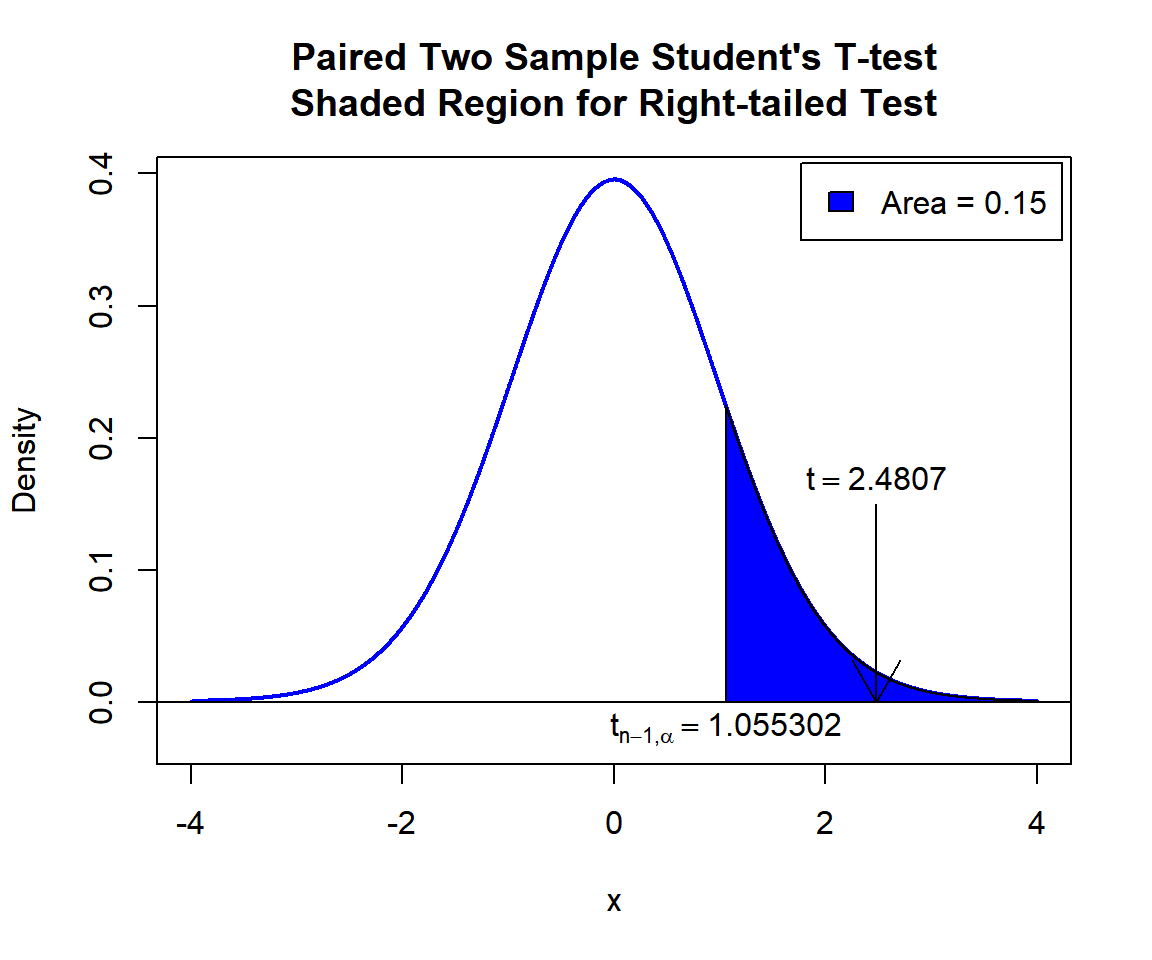
Paired Two Sample Student’s T-test Shaded Region for Right-tailed Test in R
Left Tailed Test
For "privileges" as the \(x\) group versus "learning" as the \(y\) group.
The sample means are \(\bar x =
53.1333333\) (mean(attitude$privileges)), and \(\bar y = 56.3666667\)
(mean(attitude$learning)).
For the following null hypothesis \(H_0\), and alternative hypothesis \(H_1\), with the level of significance \(\alpha=0.05\).
\(H_0:\) population mean of the paired differences is equal to 0 (\(\mu_d = 0\)).
\(H_1:\) population mean of the paired differences is less than 0 (\(\mu_d < 0\), hence one-sided).
Because the level of significance is \(\alpha=0.05\), the level of confidence is \(1 - \alpha = 0.95\).
t.test(attitude$privileges, attitude$learning,
       paired = TRUE,
       alternative = "less",
       mu = 0, conf.level = 0.95)
    Paired t-test

data:  attitude$privileges and attitude$learning
t = -1.4668, df = 29, p-value = 0.07659
alternative hypothesis: true mean difference is less than 0
95 percent confidence interval:
      -Inf 0.5120923
sample estimates:
mean difference
      -3.233333
Interpretation:
P-value: With the p-value (\(p = 0.07659\)) being greater than the level of significance 0.05, we fail to reject the null hypothesis that the population mean of the paired differences is equal to 0.
\(t\)-statistic: With test statistics value (\(t = -1.4668\)) being outside the critical region (shaded area), that is, \(t = -1.4668\) greater than \(-t_{n-1,\alpha}=\text{qt(0.05, 29)}=-1.699127\), we fail to reject the null hypothesis that the population mean of the paired differences is equal to 0.
Confidence Interval: With the null hypothesis population mean of the paired differences value (\(\mu_d = 0\)) being inside of the confidence interval, \((-\infty, 0.5120923]\), we fail to reject the null hypothesis that the population mean of the paired differences is equal to 0.
x = seq(-4, 4, 1/1000); y = dt(x, df=29)
plot(x, y, type = "l",
     xlim = c(-4, 4), ylim = c(-0.03, max(y)),
     main = "Paired Two Sample Student's T-test
Shaded Region for Left-tailed Test",
     xlab = "x", ylab = "Density",
     lwd = 2, col = "blue")
abline(h=0)
# Add shaded region and legend
point = qt(0.05, 29)
polygon(x = c(-4, x[x <= point], point),
        y = c(0, y[x <= point], 0),
        col = "blue")
legend("topright", c("Area = 0.05"),
       fill = c("blue"), inset = 0.01)
# Add critical value and t-value
arrows(0, 0.1, -1.4668, 0)
text(0, 0.12, expression(t==-1.4668))
text(-1.699127, -0.02, expression(-t[n-1][','][alpha]==-1.699127))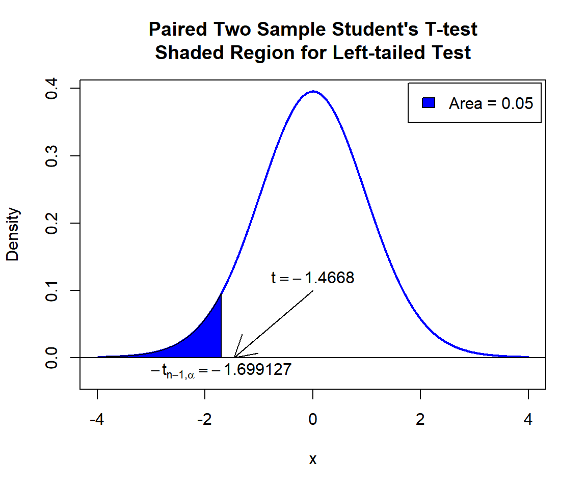
Paired Two Sample Student’s T-test Shaded Region for Left-tailed Test in R
6 Paired Two Sample T-test: Test Statistics, P-value & Degree of Freedom in R
Here for a paired two sample t-test, we show how to get the test
statistics (or t-value), p-values, and degrees of freedom from the
t.test() function in R, or by written code.
data_x = attitude$critical; data_y = attitude$raises
test_object = t.test(data_x, data_y,
                     paired = TRUE,
                     alternative = "two.sided",
                     mu = 0, conf.level = 0.95)
test_object
    Paired t-test

data:  data_x and data_y
t = 4.8969, df = 29, p-value = 3.378e-05
alternative hypothesis: true mean difference is not equal to 0
95 percent confidence interval:
  5.901069 14.365598
sample estimates:
mean difference
       10.13333
To get the test statistic or t-value:
\[t = \frac{\bar d - d_0}{s_d/ \sqrt{n}} = \frac{(\bar x - \bar y) - d_0}{s_d/ \sqrt{n}},\]
       t
4.896904 [1] 4.896904Same as:
[1] 4.896904To get the p-value:
Two-tailed: For positive test statistic (\(t^+\)), and negative test statistic (\(t^-\)).
\(Pvalue = 2*P(t_{n-1}>t^+)\) or \(Pvalue = 2*P(t_{n-1}<t^-)\).
One-tailed: For right-tail, \(Pvalue = P(t_{n-1}>t)\) or for left-tail, \(Pvalue = P(t_{n-1}<t)\).
[1] 3.378286e-05Same as:
Note that the p-value depends on the \(\text{test statistics}\) (4.8969) and \(\text{degrees of freedom}\) (29). We also
use the distribution function pt() for the Student’s
t-distribution in R.
[1] 3.378326e-05[1] 3.378326e-05One-tailed example:
To get the degrees of freedom:
The degrees of freedom are \(n-1\).
df
29 [1] 29Same as:
[1] 297 Paired Two Sample T-test: Estimates, Standard Error & Confidence Interval in R
Here for a paired two sample t-test, we show how to get the sample
means, standard error estimate, and confidence interval from the
t.test() function in R, or by written code.
data_x = attitude$learning; data_y = attitude$privileges
test_object = t.test(data_x, data_y,
                     paired = TRUE,
                     alternative = "two.sided",
                     mu = 0, conf.level = 0.9)
test_object
    Paired t-test

data:  data_x and data_y
t = 1.4668, df = 29, p-value = 0.1532
alternative hypothesis: true mean difference is not equal to 0
90 percent confidence interval:
 -0.5120923  6.9787590
sample estimates:
mean difference
       3.233333
To get the point estimate or sample mean of differences:
\[\bar d = \frac{1}{n}\sum_{i=1}^{n} (x_i - y_i).\]
mean difference
3.233333 [1] 3.233333Same as:
[1] 3.233333To get the standard error estimate:
\[\widehat {SE} = s_d/ \sqrt{n}.\]
[1] 2.204324Same as:
[1] 2.204324To get the confidence interval for \(\mu_d = \mu_x - \mu_y\):
For two-tailed: \[CI = \left[\bar d - t_{n-1,\alpha/2}*\frac{s_d}{\sqrt n} \;,\; \bar d + t_{n-1,\alpha/2}*\frac{s_d}{\sqrt n} \right].\]
For right one-tailed: \[CI = \left[\bar d - t_{n-1,\alpha}*\frac{s_d}{\sqrt n} \;,\; \infty \right).\]
For left one-tailed: \[CI = \left(-\infty \;,\; \bar d + t_{n-1,\alpha}*\frac{s_d}{\sqrt n} \right].\]
[1] -0.5120923  6.9787590
attr(,"conf.level")
[1] 0.9[1] -0.5120923 6.9787590Same as:
Note that the critical values depend on the \(\alpha\) (0.1) and \(\text{degrees of freedom}\) (29).
diff = data_x-data_y
alpha = 0.1; df = length(diff)-1
SE = sd(diff)/sqrt(length(diff))
l = mean(diff) - qt(1-alpha/2, df)*SE
u = mean(diff) + qt(1-alpha/2, df)*SE
c(l, u)
[1] -0.5120923 6.9787590One-tailed example:
The feedback form is a Google form but it does not collect any personal information.
Please click on the link below to go to the Google form.
Thank You!
Go to Feedback Form
Copyright © 2020 - 2026. All Rights Reserved by Stats Codes