Linear Regression in R
Here, we discuss linear regression in R with interpretations, including coefficients, r-squared, and p-values.
Linear regression (or ordinary least squares) in R can be performed
with the lm() function from the "stats" package in the base
version of R.
Linear regression can be used to study the linear relationship, if one exists, between a dependent variable \((y)\) and an independent variable \((x)\).
For multiple independent variables, see multiple regression.
The linear regression framework is based on the theoretical assumption that: \[y = \alpha + \beta x + \varepsilon,\]
where \(\varepsilon\) represents the error terms that are 1) independent, 2) normal distributed, 3) have constant variance, and 4) have mean zero.
The linear regression model estimates the true coefficient, \(\beta\), as \(\widehat \beta\), and the true intercept,
\(\alpha\), as \(\widehat \alpha\).
Then for any \(x\) value, these two are used to predict or
estimate the true \(y\), as \(\widehat y\), with the equation below:
\[\widehat y = \widehat \alpha + \widehat \beta x ,\] where for \(n\) sample data pairs \(\{(x_i, y_i), i = 1, ..., n\}\), \(\bar{x}\) and \(\bar{y}\) as sample means,
\[\begin{align} \widehat\beta &= \frac{ \sum_{i=1}^n (x_i - \bar{x})(y_i - \bar{y}) }{ \sum_{i=1}^n (x_i - \bar{x})^2 }, \\ \widehat\alpha & = \bar{y} - \widehat\beta\,\bar{x}. \end{align}\]
Sample Steps to Run a Regression Model:
# Create the data samples for the regression model
# Values are paired based on matching position in each sample

y = c(6.9, 5.7, 7.9, 9.6, 5.1, 8.2, 8.6, 9.4)
x = c(2.7, 2.2, 3.6, 4.3, 2.6, 3.7, 3.8, 4.0)
df_data = data.frame(y, x)
df_data

# Run the regression model

model = lm(y ~ x)
summary(model)

#or

model = lm(y ~ x, data = df_data)
summary(model)
y x
1 6.9 2.7
2 5.7 2.2
3 7.9 3.6
4 9.6 4.3
5 5.1 2.6
6 8.2 3.7
7 8.6 3.8
8 9.4 4.0
Call:
lm(formula = y ~ x)

Residuals:
     Min       1Q   Median       3Q      Max
-0.99782 -0.19638  0.00295  0.41217  0.59533

Coefficients:
            Estimate Std. Error t value Pr(>|t|)
(Intercept)   0.7199     0.9392   0.767 0.472445
x             2.0684     0.2733   7.568 0.000276 ***
---
Signif. codes:  0 '***' 0.001 '**' 0.01 '*' 0.05 '.' 0.1 ' ' 1

Residual standard error: 0.5479 on 6 degrees of freedom
Multiple R-squared:  0.9052,    Adjusted R-squared:  0.8894
F-statistic: 57.28 on 1 and 6 DF, p-value: 0.0002765| Argument | Usage |
| y ~ x | y is the dependent sample, and x is the independent sample |
| data | The dataframe object that contains the dependent and independent variables |
Creating Regression Summary Object and Model Object:
# Create data
x = rnorm(100, 20, 2)
y = 2 + 5*x + rnorm(100, 0, 1)

# Create objects
reg_summary = summary(lm(y ~ x))
reg_model = lm(y ~ x) Estimate Std. Error t value Pr(>|t|)
(Intercept) 2.298004 1.02674230 2.23815 2.747466e-02
x 4.986958 0.05188795 96.11012 8.741521e-99(Intercept) x
2.298004 4.986958 (Intercept) x
2.298004 4.986958 There are more examples in the table below.
| Regression Component | Usage |
| reg_summary$coefficients | The estimated intercept and beta values: their standard error, t-value and p-value |
| reg_summary$residuals | The regression model residuals |
| reg_summary$r.squared | The model r-squared value |
| reg_summary$adj.r.squared | The model adjusted r-squared value |
| reg_summary$fstatistic | The f-statistic and the degrees of freedom |
| reg_summary$sigma | The model residuals standard error |
| reg_model$coefficients | The estimated intercept and beta values |
| reg_model$residuals | The regression model residuals |
| reg_model$fitted.values | The predicted y values |
| reg_model$df.residual | The degrees of freedom of the residuals |
| reg_model$model | The model dataframe |
1 Steps to Running a Regression in R
Using the first 10 rows of the "faithful" data from the "datasets" package below:
   eruptions waiting
1      3.600      79
2      1.800      54
3      3.333      74
4      2.283      62
5      4.533      85
6      2.883      55
7      4.700      88
8      3.600      85
9      1.950      51
10     4.350      85
NOTE: The dependent variable is "waiting", and the independent variable is "eruptions".
1.1 Check for Linear Relationship
Use a scatter plot to visually check for a linear relationship.
data_f = faithful[1:10,]
x = data_f$eruptions
y = data_f$waiting
plot(x, y,
     main = "Scatter Plot with Regression and Lowess Lines in R")
abline(lm(y ~ x), col = "blue")
lines(lowess(x, y), col = "red", lty = "dashed")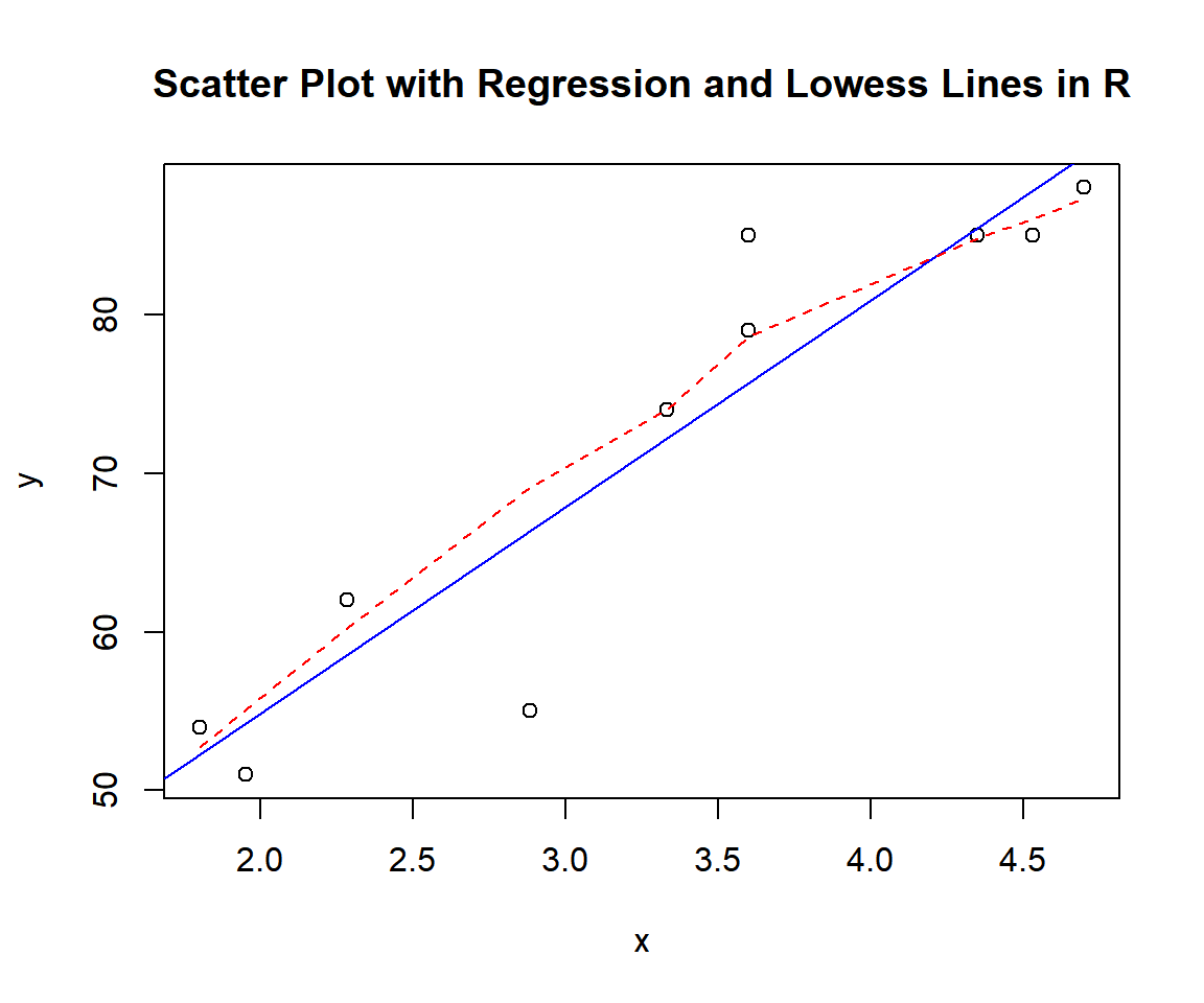
Scatter Plot with Regression and Lowess Lines in R
The appearance of the scatter plot suggests a strong linear relationship.
1.2 Run the Regression
Run the linear regression model using the lm() function,
and print the results using the summary() function.
data_f = faithful[1:10,]
eruptions = data_f$eruptions
waiting = data_f$waiting
model = lm(waiting ~ eruptions)
summary(model)
Or:
Call:
lm(formula = waiting ~ eruptions, data = data_f)

Residuals:
     Min       1Q   Median       3Q      Max
-11.3298  -2.6033   0.6707   2.9552   9.3362

Coefficients:
            Estimate Std. Error t value Pr(>|t|)
(Intercept)   28.798      6.296   4.574  0.00182 **
eruptions     13.018      1.824   7.137 9.83e-05 ***
---
Signif. codes:  0 '***' 0.001 '**' 0.01 '*' 0.05 '.' 0.1 ' ' 1

Residual standard error: 5.781 on 8 degrees of freedom
Multiple R-squared:  0.8643,    Adjusted R-squared:  0.8473
F-statistic: 50.94 on 1 and 8 DF,  p-value: 9.832e-05
1.3 Interpretation of the Results
- Coefficients:
- The estimated intercept (\(\widehat \alpha\)) is \(\text{summary(model)\$coefficients[1, 1]}\) \(= 28.798\).
- The estimated coefficient for \(x\) (\(\widehat \beta\)) is \(\text{summary(model)\$coefficients[2, 1]}\) \(= 13.018\).
- P-values:
For level of significance, \(\alpha = 0.05\).- The p-value for the intercept is \(\text{summary(model)\$coefficients[1, 4]}\) \(= 0.0018165\). Since the p-value is less than \(0.05\), we say that the intercept is statistically significantly different from zero.
- The p-value for the independent variable, \(x\) (eruptions), is \(\text{summary(model)\$coefficients[2, 4]}\)
\(= 9.83\times 10^{-5}\). Since the
p-value is less than \(0.05\), we say
that the independent variable is a statistically significant predictor
of the dependent variable \(y\)
(waitings).
If the p-value were higher than the chosen level of significance, we would have concluded that the independent variable is NOT a statistically significant predictor of the dependent variable.
- R-squared:
The r-squared value is \(\text{summary(model)\$r.squared}\) \(= 0.864\).
This means that the model, using the independent variable, \(x\) (eruptions), explains \(86.4\%\) of the variations in the dependent variable \(y\) (waitings) from the sample mean of \(y\), \(\bar y\).
1.4 Prediction and Estimation
To predict or estimate \(y\) for any \(x\), we can use \(y = 28.798 + 13.018 x\).
For example, for \(x = 5\), \(y = 28.798+ 13.018 \times 5\) \(= 93.888\).
The feedback form is a Google form but it does not collect any personal information.
Please click on the link below to go to the Google form.
Thank You!
Go to Feedback Form
Copyright © 2020 - 2026. All Rights Reserved by Stats Codes