1 Table of Chi-Squared Distribution Functions in R
2 Plot of Chi-Squared Distributions in R
3 Examples for Setting Parameters for Chi-Squared Distributions in R
4 rchisq(): Random Sampling from Chi-Squared Distributions in R
5 dchisq(): Probability Density Function for Chi-Squared Distributions in R
6 pchisq(): Cumulative Distribution Function for Chi-Squared Distributions in R
7 qchisq(): Derive Quantile for Chi-Squared Distributions in R

Here, we discuss chi-squared distribution functions in R, plots, parameter setting, random sampling, density, cumulative distribution and quantiles.

The chi-squared distribution with parameter \(\tt{degrees\;of\;freedom} = k\) has probability density function (pdf) formula as:

\[f(x) = \begin{cases} \dfrac{x^{(k/2) -1} e^{-x/2}}{2^{k/2} \Gamma\left(k/2 \right)}, & x > 0; \\ 0 \;, & \text{otherwise}. \end{cases},\] where \(k \geq 0\), and \(\Gamma\) is the \(\tt{gamma\;function}\).

The mean is \(k\), and the variance is \(2k\).

1 Table of Chi-Squared Distribution Functions in R

The table below shows the functions for chi-squared distributions in R.

Table of Chi-Squared Distribution Functions in R
Function	Usage
rchisq(n, df, ncp=0)	Simulate a random sample with \(n\) observations
dchisq(x, df, ncp=0)	Calculate the probability density at the point \(x\)
pchisq(q, df, ncp=0)	Calculate the cumulative distribution at the point \(q\)
qchisq(p, df, ncp=0)	Calculate the quantile value associated with \(p\)

The examples here are central chi-squared distributions, hence, the "ncp" argument is excluded in the examples below.

However, for non-central chi-squared distributions, you can set the argument of the non-centrality parameter value to a non-zero value as ncp = 0 is central. For example:

pchisq(4.3, df = 6, ncp = 0)

[1] 0.3638509

# It is the same as:
pchisq(4.3, df = 6)

[1] 0.3638509

2 Plot of Chi-Squared Distributions in R

Single distribution:

Below is a plot of the chi-squared distribution function with \(\tt{df}=5\).

x = seq(0, 20, 1/1000); y = dchisq(x, 5)
plot(x, y, type = "l",
     xlim = c(0, 20), ylim = c(0, max(y)),
     main = "Probability Density Function of Chi-Squared Distribution (5)",
     xlab = "x", ylab = "Density",
     lwd = 2, col = "blue")
# Add legend
legend("topright", "df = 5",
       lwd = 2,
       col = "blue",
       bty = "n")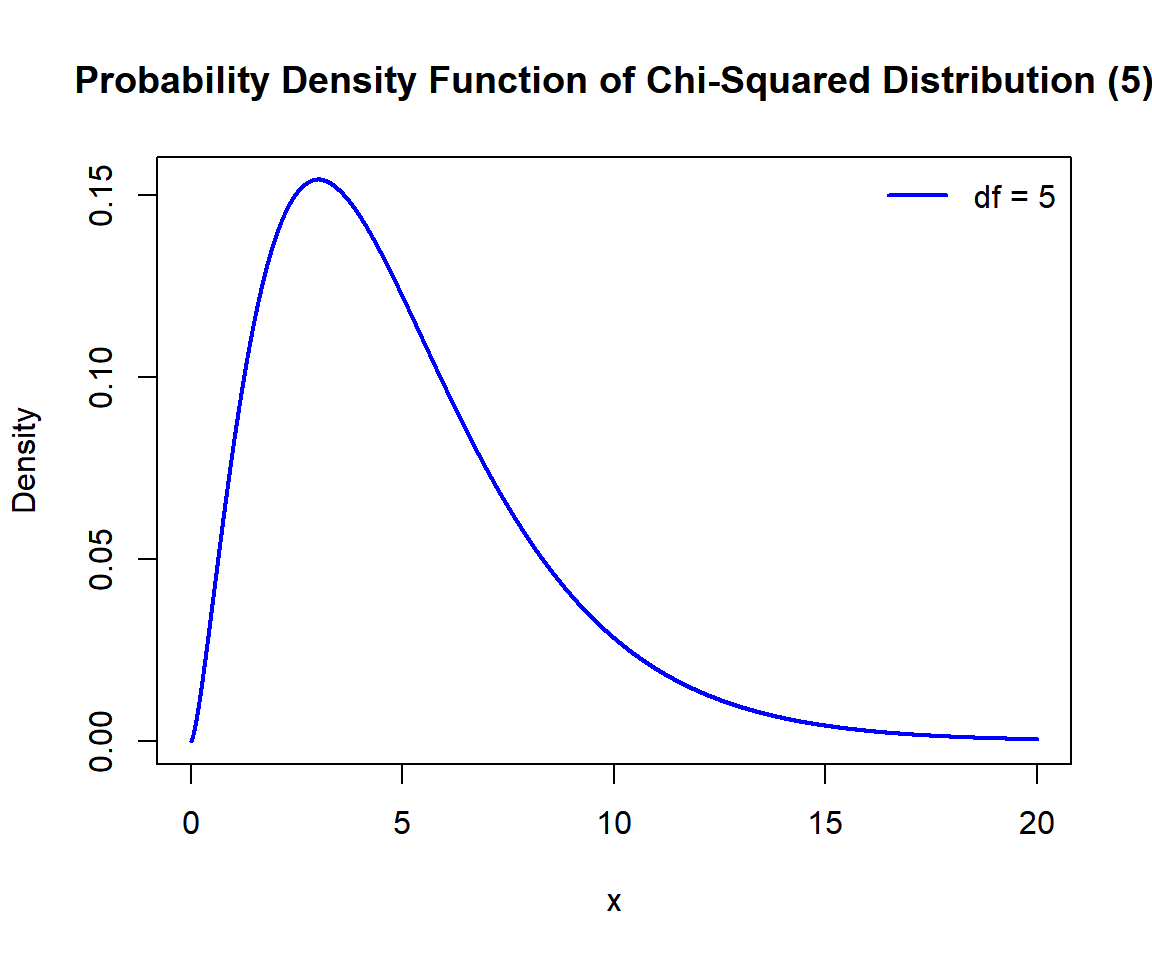

Probability Density Function (PDF) of a Chi-Squared Distribution in R

Multiple distributions:

Below is a plot of multiple chi-squared distribution functions in one graph.

x1 = seq(0, 20, 1/1000); y1 = dchisq(x1, 2)
x2 = seq(0, 20, 1/1000); y2 = dchisq(x2, 5)
x3 = seq(0, 20, 1/1000); y3 = dchisq(x3, 10)
plot(x1, y1, type = "l",
     xlim = c(0, 20), ylim = range(c(y1, y2, y3)),
     main = "Probability Density Functions of Chi-Squared Distributions",
     xlab = "x", ylab = "Density",
     lwd = 2, col = "blue")
points(x2, y2, type = "l", lwd = 2, col = "red")
points(x3, y3, type = "l", lwd = 2, col = "green")
# Add legend
legend("topright", c("df = 2",
                    "df = 5",
                    "df = 10"),
       lwd = c(2, 2, 2),
       col = c("blue", "red", "green"),
       bty = "n")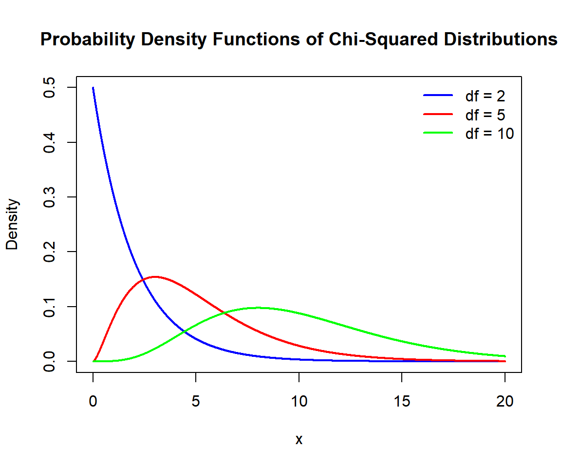

Probability Density Functions (PDFs) of Chi-Squared Distributions in R

3 Examples for Setting Parameters for Chi-Squared Distributions in R

To set the parameter for the chi-squared distribution function, with \(\tt{degrees\;of\;freedom} = 8\).

For example, for dchisq(), the following are the same:

dchisq(1.25, 8)

[1] 0.01088992

dchisq(1.25, df = 8)

[1] 0.01088992

4 rchisq(): Random Sampling from Chi-Squared Distributions in R

Sample 800 observations from the chi-squared distribution with \(\tt{degrees\;of\;freedom} = 6\):

rchisq(800, 6)

set.seed(1234) # Line allows replication (use any number).
sample = rchisq(800, 6)
hist(sample,
     main = "Histogram of 800 Observations from Chi-Squared
Distribution with Degrees of Freedom = 6",
     xlab = "x",
     col = "deepskyblue", border = "white")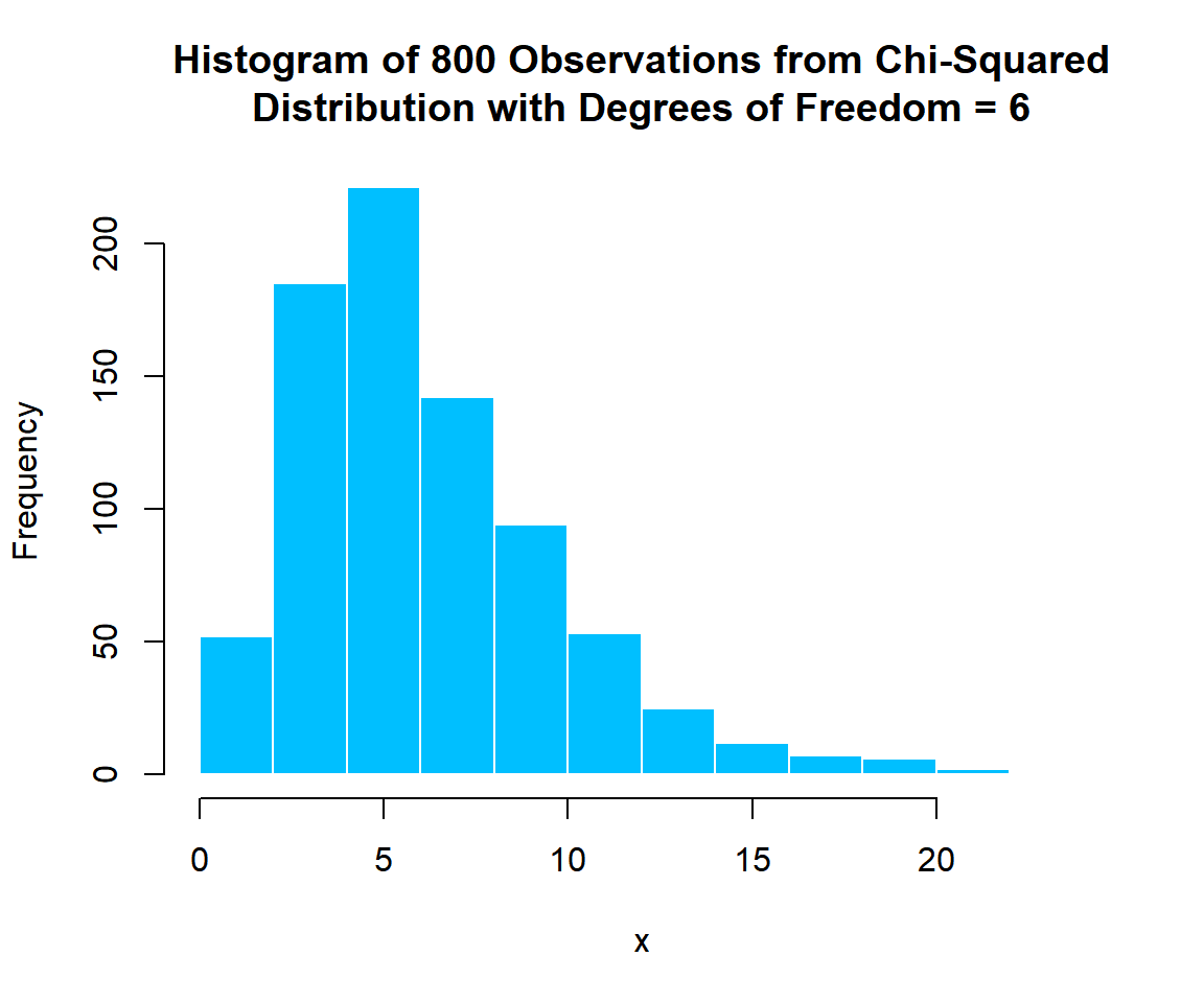

Histogram of Chi-Squared Distribution (6) Random Sample in R

5 dchisq(): Probability Density Function for Chi-Squared Distributions in R

Calculate the density at \(x = 4.5\), in the chi-squared distribution with \(\tt{degrees\;of\;freedom} = 4\):

dchisq(4.5, 4)

[1] 0.1185741

x = seq(0, 20, 1/1000); y = dchisq(x, 4)
plot(x, y, type = "l",
     xlim = c(0, 20), ylim = c(0, max(y)),
     main = "Probability Density Function of Chi-Squared
Distribution with Degrees of Freedom = 4",
     xlab = "x", ylab = "Density",
     lwd = 2, col = "blue")
# Add lines
segments(4.5, -1, 4.5, 0.1185741)
segments(-1, 0.1185741, 4.5, 0.1185741)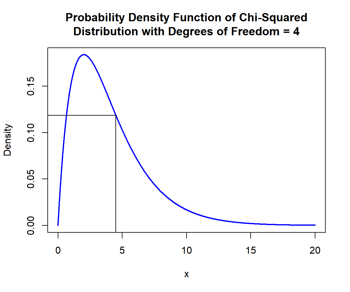

Probability Density Function (PDF) of Chi-Squared Distribution (4) in R

6 pchisq(): Cumulative Distribution Function for Chi-Squared Distributions in R

Calculate the cumulative distribution at \(x = 14.6\), in the chi-squared distribution with \(\tt{degrees\;of\;freedom} = 7\). That is, \(P(X \le 14.6)\):

pchisq(14.6, 7)

[1] 0.9585173

x = seq(0, 25, 1/1000); y = pchisq(x, 7)
plot(x, y, type = "l",
     xlim = c(0, 25), ylim = c(0,1),
     main = "Cumulative Distribution Function of Chi-Squared
Distribution with Degrees of Freedom = 7",
     xlab = "x", ylab = "Cumulative Distribution",
     lwd = 2, col = "blue")
# Add lines
segments(14.6, -1, 14.6, 0.9585173)
segments(-1, 0.9585173, 14.6, 0.9585173)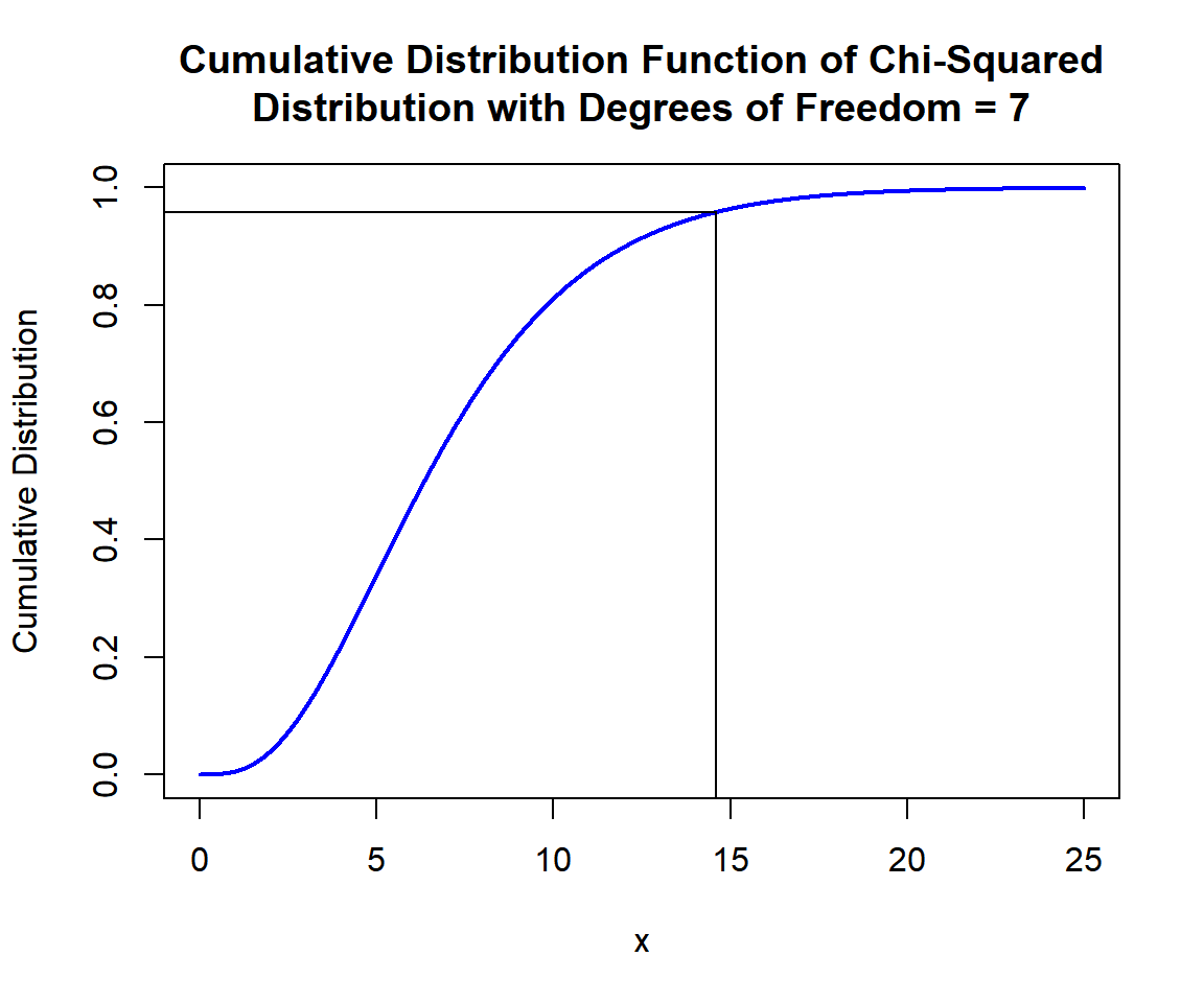

Cumulative Distribution Function (CDF) of Chi-Squared Distribution (7) in R

x = seq(0, 25, 1/1000); y = dchisq(x, 7)
plot(x, y, type = "l",
     xlim = c(0, 25), ylim = c(0, max(y)),
     main = "Cumulative Distribution Function of Chi-Squared
Distribution with Degrees of Freedom = 7",
     xlab = "x", ylab = "Density",
     lwd = 2, col = "blue")
# Add shaded region and legend
point = 14.6
polygon(x = c(x[x <= point], point),
        y = c(y[x <= point], 0),
        col = "limegreen")
legend("topright", c("Area = 0.9585173"),
       fill = c("limegreen"),
       inset = 0.01)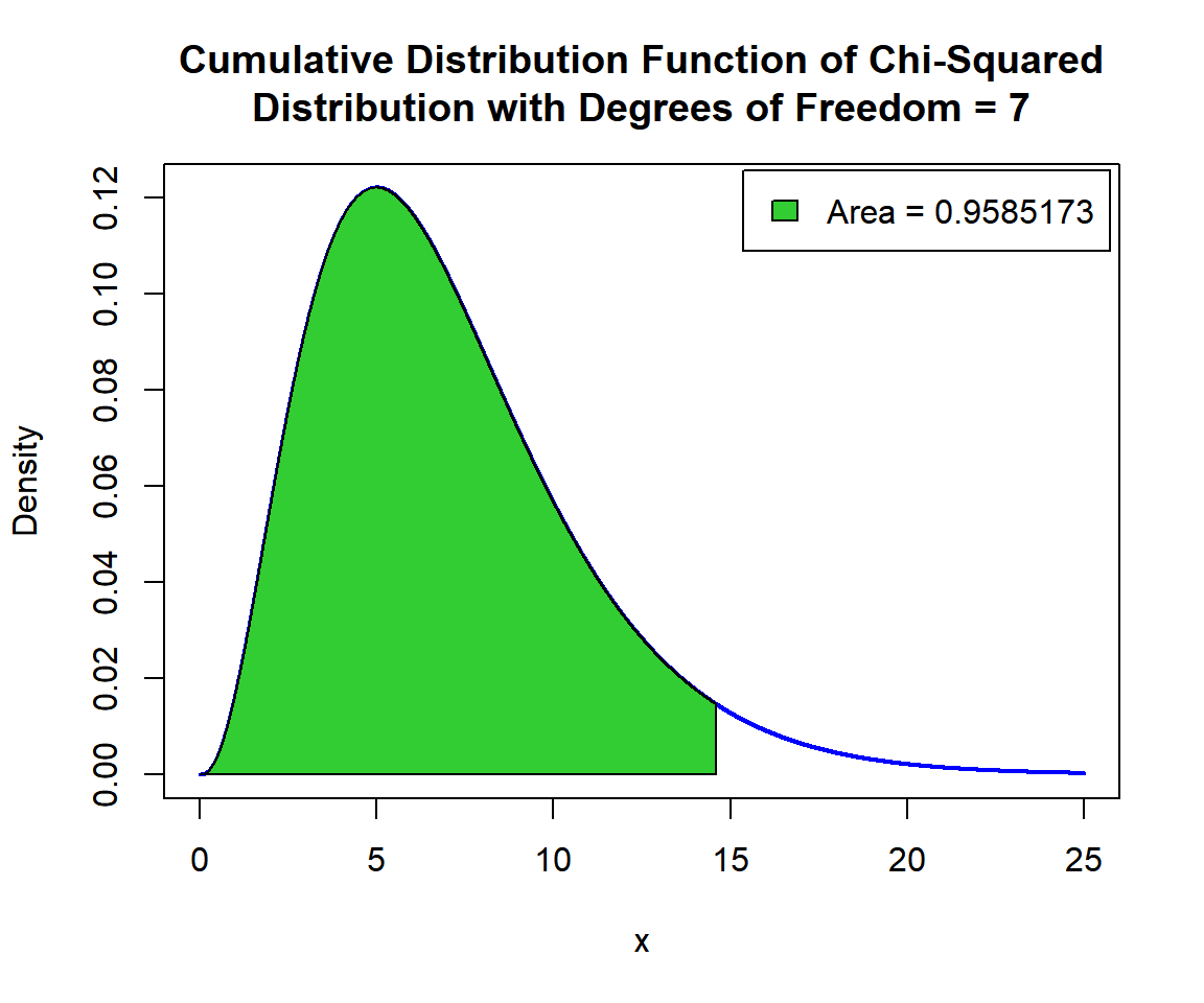

Shaded Probability Density Function (PDF) of Chi-Squared Distribution (7) in R

For upper tail, at \(x = 14.6\), that is, \(P(X \ge 14.6) = 1 - P(X \le 14.6)\), set the "lower.tail" argument:

pchisq(14.6, 7, lower.tail = FALSE)

[1] 0.04148266

x = seq(0, 25, 1/1000); y = dchisq(x, 7)
plot(x, y, type = "l",
     xlim = c(0, 25), ylim = c(0, max(y)),
     main = "Shaded Upper Region: Probability Density Function of
Chi-Squared Distribution with Degrees of Freedom = 7",
     xlab = "x", ylab = "Density",
     lwd = 2, col = "blue")
# Add shaded region and legend
point = 14.6
polygon(x = c(point, x[x >= point]),
        y = c(0, y[x >= point]),
        col = "limegreen")
legend("topright", c("Area = 0.04148266"),
       fill = c("limegreen"),
       inset = 0.01)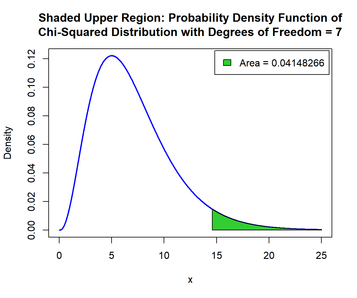

Shaded Upper Region: Probability Density Function (PDF) of Chi-Squared Distribution (7) in R

7 qchisq(): Derive Quantile for Chi-Squared Distributions in R

Derive the quantile for \(p = 0.8\), in the chi-squared distribution with \(\tt{degrees\;of\;freedom} = 3\). That is, \(x\) such that, \(P(X \le x)=0.8\):

qchisq(0.8, 3)

[1] 4.641628

x = seq(0, 15, 1/1000); y = pchisq(x, 3)
plot(x, y, type = "l",
     xlim = c(0, 15), ylim = c(0,1),
     main = "Cumulative Distribution Function of Chi-Squared
Distribution with Degrees of Freedom = 3",
     xlab = "x", ylab = "Cumulative Distribution",
     lwd = 2, col = "blue")
# Add lines
segments(4.641628, -1, 4.641628, 0.8)
segments(-1, 0.8, 4.641628, 0.8)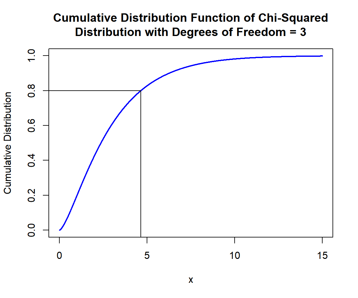

Cumulative Distribution Function (CDF) of Chi-Squared Distribution (3) in R

x = seq(0, 15, 1/1000); y = dchisq(x, 3)
plot(x, y, type = "l",
     xlim = c(0, 15), ylim = c(0, max(y)),
     main = "Probability Density Function of Chi-Squared
Distribution with Degrees of Freedom = 3",
     xlab = "x", ylab = "Density",
     lwd = 2, col = "blue")
# Add shaded region and legend
point = 4.641628
polygon(x = c(x[x <= point], point),
        y = c(y[x <= point], 0),
        col = "limegreen")
legend("topright", c("Area = 0.8"),
       fill = c("limegreen"),
       inset = 0.01)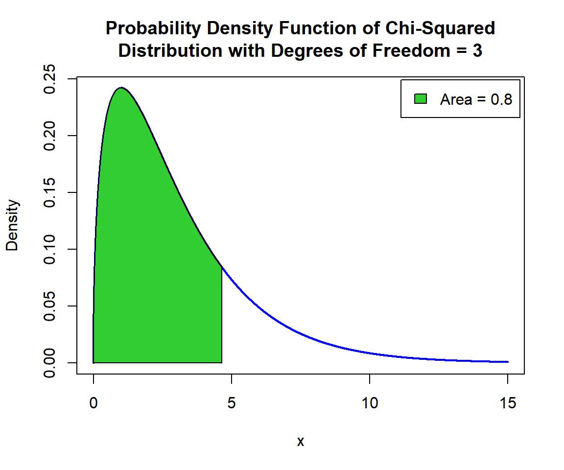

Shaded Probability Density Function (PDF) of Chi-Squared Distribution (3) in R

For upper tail, for \(p = 0.2\), that is, \(x\) such that, \(P(X \ge x)=0.2\):

qchisq(0.2, 3, lower.tail = FALSE)

[1] 4.641628

x = seq(0, 15, 1/1000); y = dchisq(x, 3)
plot(x, y, type = "l",
     xlim = c(0, 15), ylim = c(0, max(y)),
     main = "Shaded Upper Region: Probability Density Function of
Chi-Squared Distribution with Degrees of Freedom = 3",
     xlab = "x", ylab = "Density",
     lwd = 2, col = "blue")
# Add shaded region and legend
point = 4.641628
polygon(x = c(point, x[x >= point]),
        y = c(0, y[x >= point]),
        col = "limegreen")
legend("topright", c("Area = 0.2"),
       fill = c("limegreen"),
       inset = 0.01)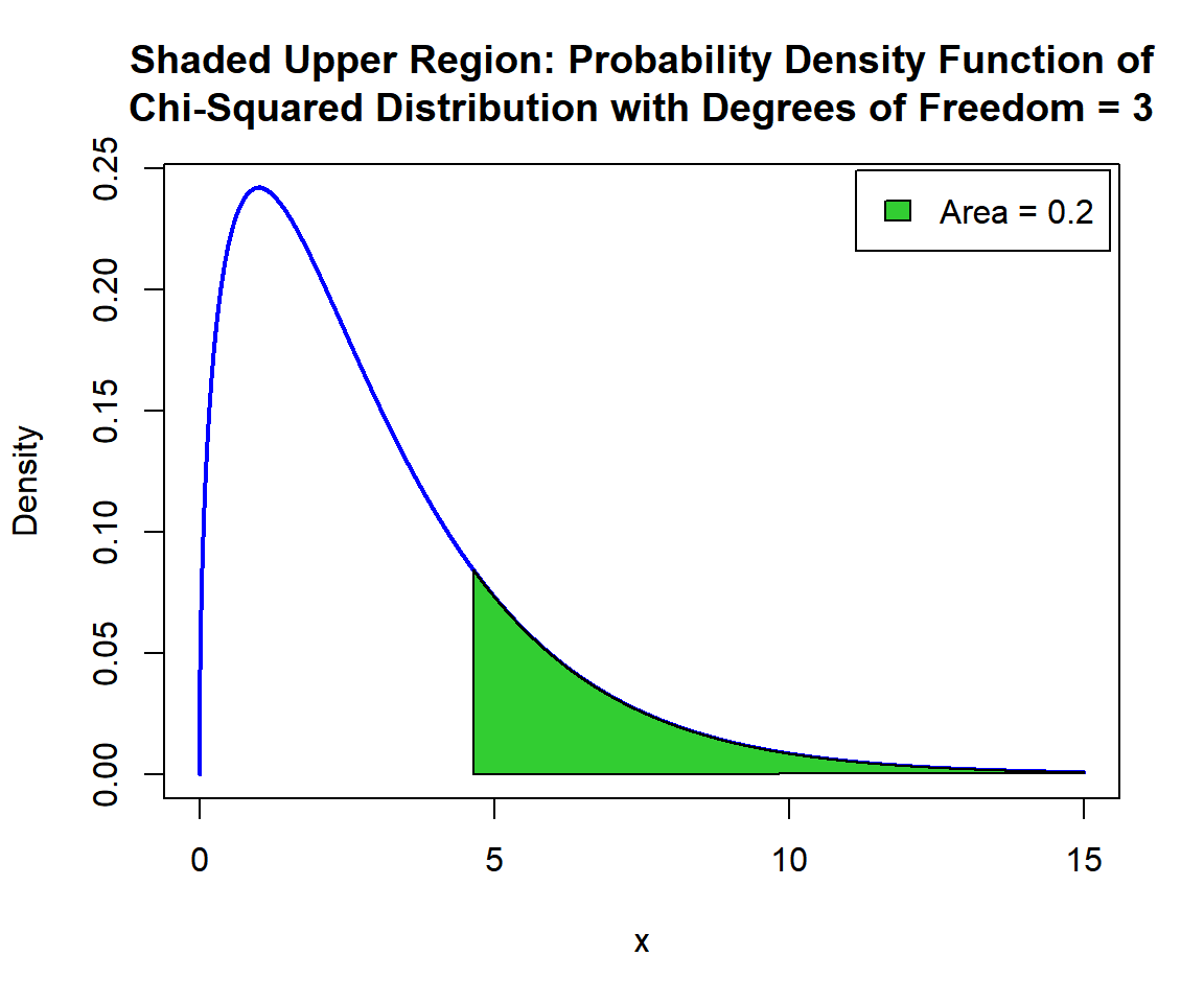

Shaded Upper Region: Probability Density Function (PDF) of Chi-Squared Distribution (3) in R