Student’s t Distributions in R
- 1 Table of Student’s t Distribution Functions in R
- 2 Plot of Student’s t Distributions in R
- 3 Examples for Setting Parameters for Student’s t Distributions in R
- 4 rt(): Random Sampling from Student’s t Distributions in R
- 5 dt(): Probability Density Function for Student’s t Distributions in R
- 6 pt(): Cumulative Distribution Function for Student’s t Distributions in R
- 7 qt(): Derive Quantile for Student’s t Distributions in R
Here, we discuss Student’s t distribution functions in R, plots, parameter setting, random sampling, density, cumulative distribution and quantiles.
The Student’s t distribution with parameter \(\tt{degree\;of\;freedom}=\nu\) has probability density function (pdf) formula as:
\[\begin{align} f(x)& =\frac{\Gamma \left(\frac{\nu+1}{2} \right)} {\sqrt{\nu\pi}\,\Gamma \left(\frac{\nu}{2} \right)} \left(1+\frac{x^2}{\nu} \right)^{-\frac{\nu+1}{2}} \\ & = \frac{1}{\sqrt{\nu}\,\mathrm{B} (\frac{1}{2}, \frac{\nu}{2})} \left(1+\frac{x^2}\nu \right)^{-\frac{\nu+1}{2}},\end{align}\] for \(x\in\mathbb{R}\), where \(\nu > 0\),
\(\Gamma\) is the \(\tt{gamma\;function}\), and \(\mathrm{B}\) is the \(\tt{beta\;function}\).
The mean is \(0\) for \(\nu > 1\), otherwise undefined,
the variance is \(\frac{\nu}{\nu-2}\) for \(\nu > 2\); \(\infty\) for \(1 < \nu \le 2\); and otherwise undefined.
See also probability distributions and plots and charts.
1 Table of Student’s t Distribution Functions in R
The table below shows the functions for Student’s t distributions in R.
| Function | Usage |
| rt(n, df, ncp) | Simulate a random sample with \(n\) observations |
| dt(x, df, ncp) | Calculate the probability density at the point \(x\) |
| pt(q, df, ncp) | Calculate the cumulative distribution at the point \(q\) |
| qt(p, df, ncp) | Calculate the quantile value associated with \(p\) |
The examples here are central Student’s t distributions, hence, the "ncp" argument is excluded in the examples below.
However, for non-central Student’s t distributions,
you can set the argument of the non-centrality parameter value to a
non-zero value as ncp = 0 is central. For example:
[1] 0.0460441[1] 0.04604412 Plot of Student’s t Distributions in R
Single distribution:
Below is a plot of the Student’s t distribution function with \(\tt{degree\;of\;freedom\;}=35\).
x = seq(-4, 4, 1/1000); y = dt(x, 35)
plot(x, y, type = "l",
     xlim = c(-4, 4), ylim = c(0, max(y)),
     main = "Probability Density Function of Student's t Distribution (35)",
     xlab = "x", ylab = "Density",
     lwd = 2, col = "blue")
# Add line and legend
lines(c(0, 0), c(0, max(y)), col = "red")
legend("topleft", "df = 35",
       lwd = 2,
       col = "blue",
       bty = "n")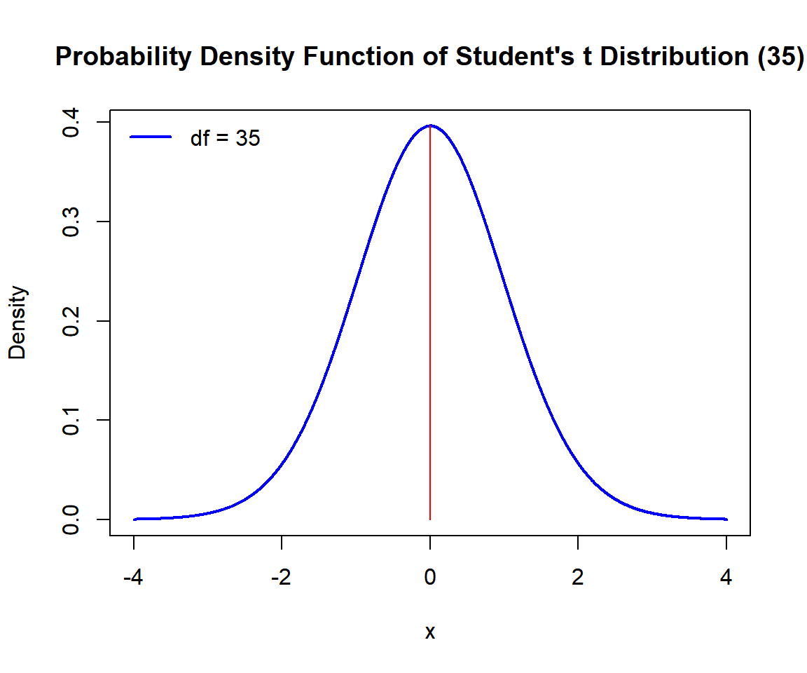
Probability Density Function (PDF) of a Student’s t Distribution in R
Multiple distributions:
Below is a plot of multiple Student’s t distribution functions in one graph.
x1 = seq(-7, 7, 1/1000); y1 = dt(x1, 60)
x2 = seq(-7, 7, 1/1000); y2 = dt(x2, 5)
x3 = seq(-7, 7, 1/1000); y3 = dt(x3, 2)
plot(x1, y1, type = "l",
     xlim = c(-7, 7), ylim = range(c(y1, y2, y3)),
     main = "Probability Density Functions of Student's t Distributions",
     xlab = "x", ylab = "Density",
     lwd = 2, col = "blue")
points(x2, y2, type = "l", lwd = 2, col = "red")
points(x3, y3, type = "l", lwd = 2, col = "green")
# Add legend
legend("topleft", c("df = 60",
                    "df = 5",
                    "df = 2"),
       lwd = c(2, 2, 2),
       col = c("blue", "red", "green"),
       bty = "n")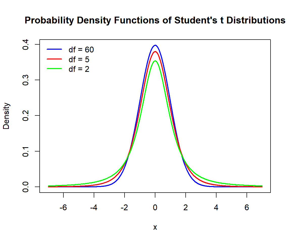
Probability Density Functions (PDFs) of Student’s t Distributions in R
3 Examples for Setting Parameters for Student’s t Distributions in R
To set the parameter for the Student’s t distribution function, with \(\tt{degrees\;of\;freedom}=15\).
For example, for pt(), the following are the same:
[1] 0.9780522[1] 0.97805224 rt(): Random Sampling from Student’s t Distributions in R
Sample 1500 observations from the Student’s t distribution with \(\tt{degree\;of\;freedom\;}=60\):
set.seed(100) # Line allows replication (use any number).
sample = rt(1500, 60)
hist(sample,
     main = "Histogram of 1500 Observations from Student's t
Distribution with 60 Degrees of Freedom",
     xlab = "x",
     col = "deepskyblue", border = "white")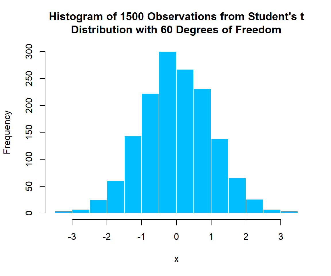
Histogram of Student’s t Distribution (60) Random Sample in R
5 dt(): Probability Density Function for Student’s t Distributions in R
Calculate the density at \(x = 1.5\), in the Student’s t distribution with with \(\tt{degree\;of\;freedom\;}=40\):
[1] 0.1291154x = seq(-4, 4, 1/1000); y = dt(x, 40)
plot(x, y, type = "l",
xlim = c(-4, 4), ylim = c(0, max(y)),
main = "Probability Density Function of Student's t Distribution
with 40 Degrees of Freedom",
xlab = "x", ylab = "Density",
lwd = 2, col = "blue")
# Add lines
segments(1.5, -1, 1.5, 0.1291154)
segments(-5, 0.1291154, 1.5, 0.1291154)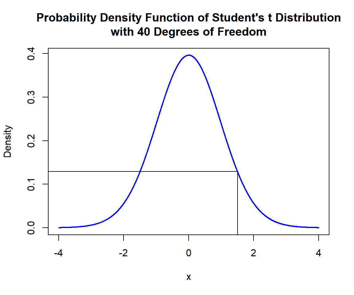
Probability Density Function (PDF) of Student’s t Distribution (40) in R
6 pt(): Cumulative Distribution Function for Student’s t Distributions in R
Calculate the cumulative distribution at \(x = 1.6\), in the Student’s t distribution with \(\tt{degree\;of\;freedom\;}=80\). That is, \(P(X \le 1.6)\):
[1] 0.9432297x = seq(-4, 4, 1/1000); y = pt(x, 80)
plot(x, y, type = "l",
xlim = c(-4, 4), ylim = c(0,1),
main = "Cumulative Distribution Function of Student's t Distribution
with 80 Degrees of Freedom",
xlab = "x", ylab = "Cumulative Distribution",
lwd = 2, col = "blue")
# Add lines
segments(1.6, -1, 1.6, 0.9432297)
segments(-5, 0.9432297, 1.6, 0.9432297)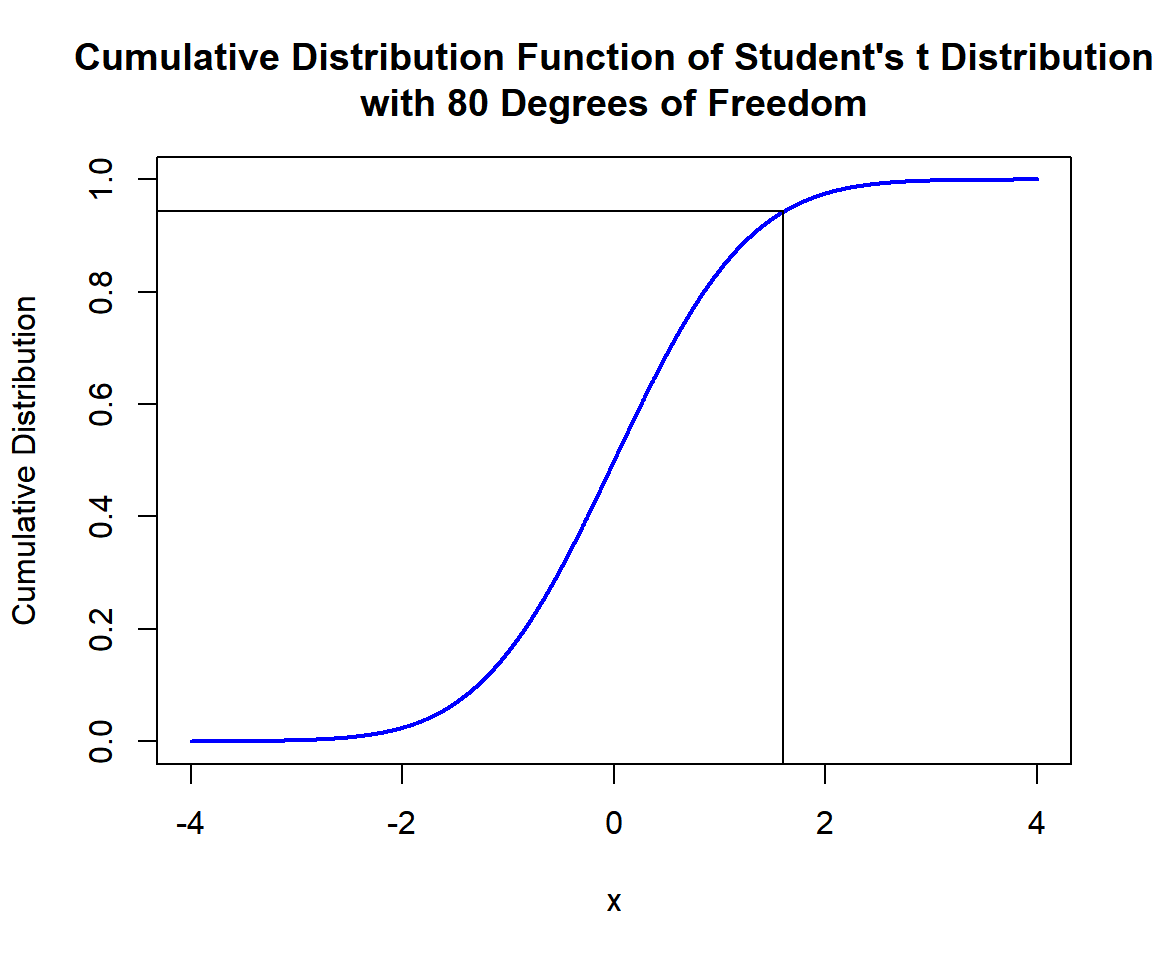
Cumulative Distribution Function (CDF) of Student’s t Distribution (80) in R
x = seq(-4, 4, 1/1000); y = dt(x, 80)
plot(x, y, type = "l",
     xlim = c(-4, 4), ylim = c(0, max(y)),
     main = "Probability Density Function of Student's t Distribution
with 80 Degrees of Freedom",
     xlab = "x", ylab = "Density",
     lwd = 2, col = "blue")
# Add shaded region and legend
point = 1.6
polygon(x = c(x[x <= point], point),
        y = c(y[x <= point], 0),
        col = "limegreen")
legend("topright", c("Area = 0.9432297"),
       fill = c("limegreen"),
       inset = 0.01)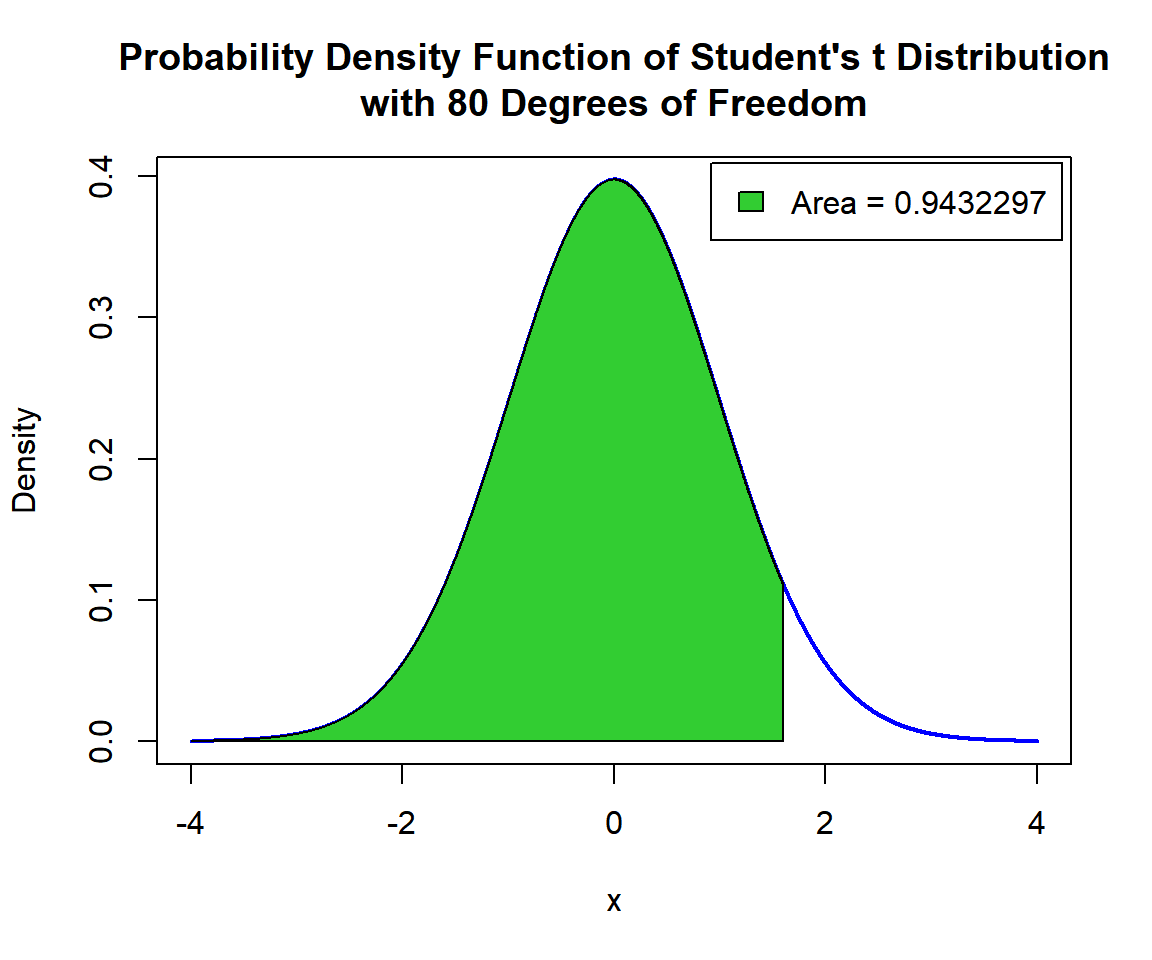
Shaded Probability Density Function (PDF) of Student’s t Distribution (80) in R
For upper tail, at \(x = 1.6\), that is, \(P(X \ge 1.6) = 1 - P(X \le 1.6)\), set the "lower.tail" argument:
[1] 0.05677031x = seq(-4, 4, 1/1000); y = dt(x, 80)
plot(x, y, type = "l",
xlim = c(-4, 4), ylim = c(0, max(y)),
main = "Shaded Upper Region: Probability Density Function of
Student's t Distribution with 80 Degrees of Freedom",
xlab = "x", ylab = "Density",
lwd = 2, col = "blue")
# Add shaded region and legend
point = 1.6
polygon(x = c(point, x[x >= point]),
y = c(0, y[x >= point]),
col = "limegreen")
legend("topright", c("Area = 0.05677031"),
fill = c("limegreen"),
inset = 0.01)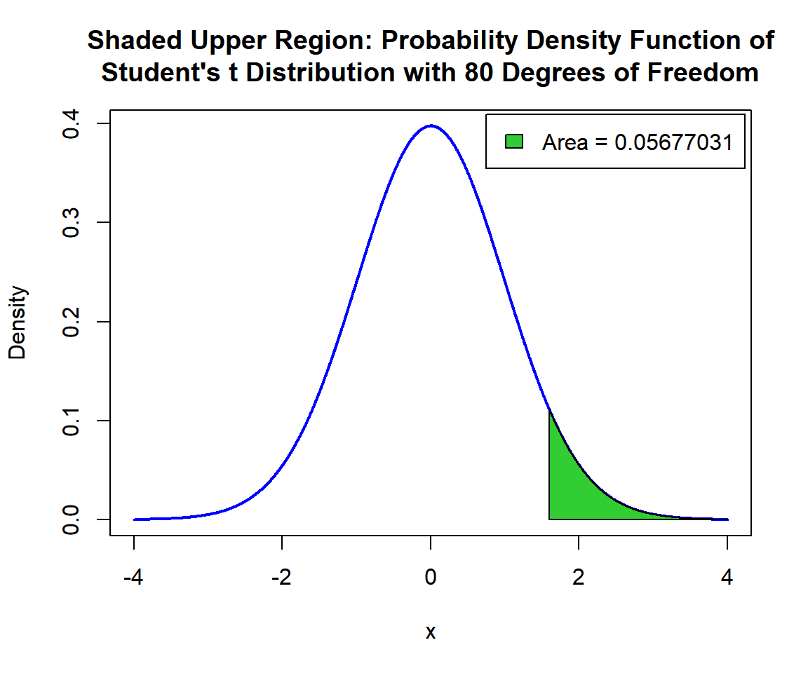
Shaded Upper Region: Probability Density Function (PDF) of Student’s t Distribution (80) in R
7 qt(): Derive Quantile for Student’s t Distributions in R
Derive the quantile for \(p = 0.9\), in the Student’s t distribution with \(\tt{degree\;of\;freedom\;}=50\). That is, \(x\) such that, \(P(X \le x)=0.9\):
[1] 1.298714x = seq(-4, 4, 1/1000); y = pt(x, 50)
plot(x, y, type = "l",
xlim = c(-4, 4), ylim = c(0,1),
main = "Cumulative Distribution Function of Student's t Distribution
with 50 Degrees of Freedom",
xlab = "x", ylab = "Cumulative Distribution",
lwd = 2, col = "blue")
# Add lines
segments(1.298714, -1, 1.298714, 0.9)
segments(-5, 0.9, 1.298714, 0.9)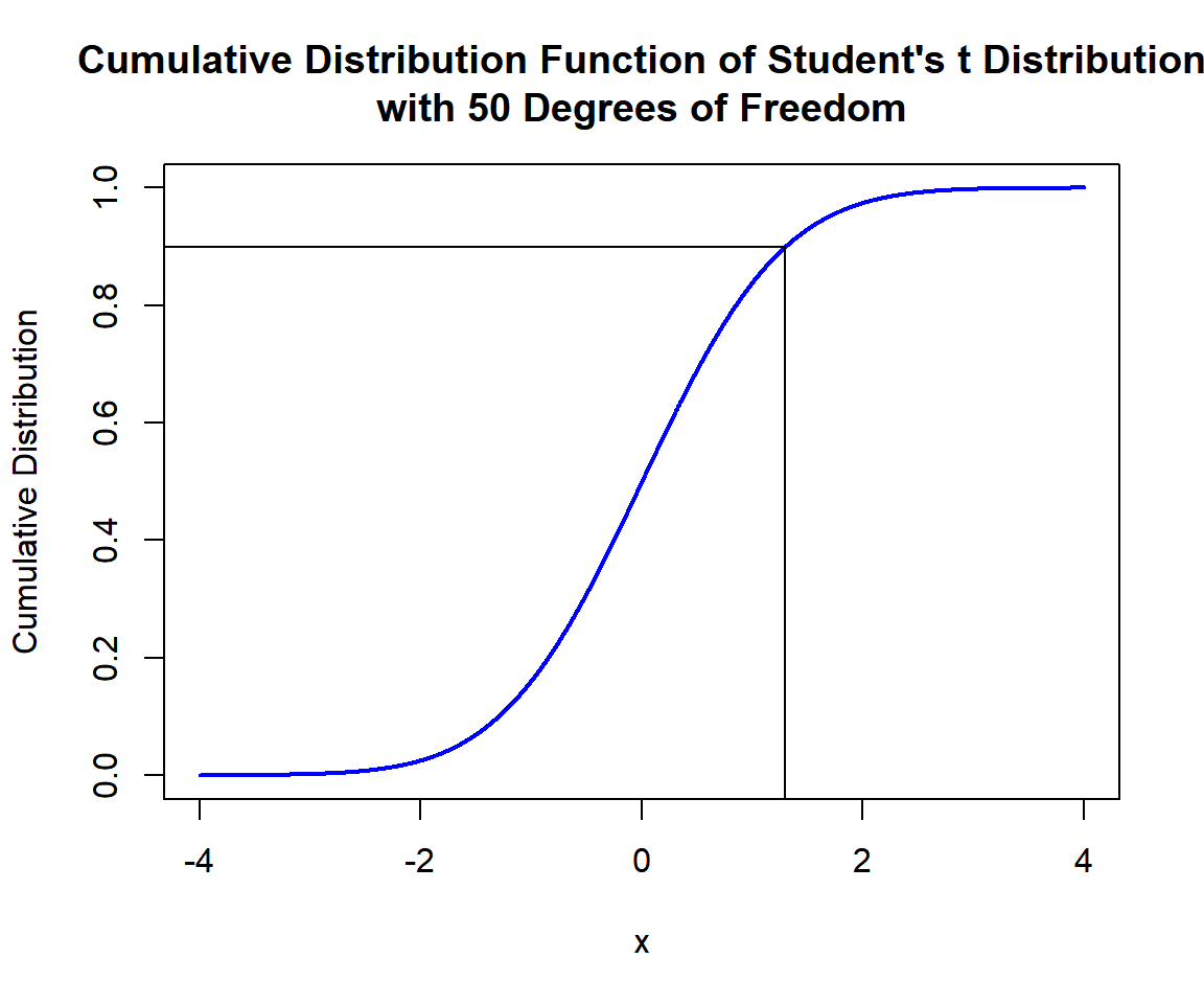
Cumulative Distribution Function (CDF) of Student’s t Distribution (50) in R
x = seq(-4, 4, 1/1000); y = dt(x, 50)
plot(x, y, type = "l",
     xlim = c(-4, 4), ylim = c(0, max(y)),
     main = "Probability Density Function of Student's t Distribution
with 50 Degrees of Freedom",
     xlab = "x", ylab = "Density",
     lwd = 2, col = "blue")
# Add shaded region and legend
point = 1.298714
polygon(x = c(x[x <= point], point),
        y = c(y[x <= point], 0),
        col = "limegreen")
legend("topright", c("Area = 0.9"),
       fill = c("limegreen"),
       inset = 0.01)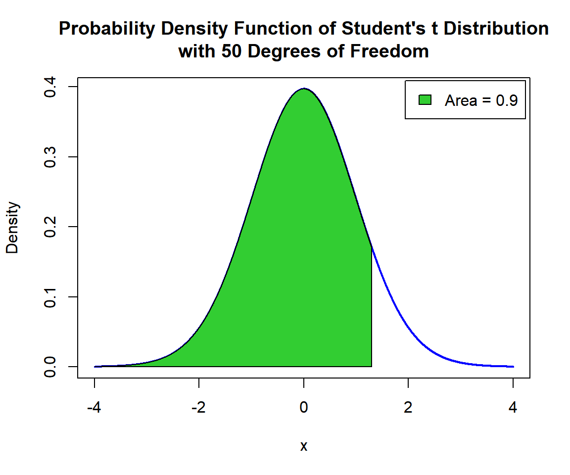
Shaded Probability Density Function (PDF) of Student’s t Distribution (50) in R
For upper tail, for \(p = 0.1\), that is, \(x\) such that, \(P(X \ge x)=0.1\):
[1] 1.298714x = seq(-4, 4, 1/1000); y = dt(x, 50)
plot(x, y, type = "l",
xlim = c(-4, 4), ylim = c(0, max(y)),
main = "Shaded Upper Region: Probability Density Function of
Student's t Distribution with 50 Degrees of Freedom",
xlab = "x", ylab = "Density",
lwd = 2, col = "blue")
# Add shaded region and legend
point = 1.298714
polygon(x = c(point, x[x >= point]),
y = c(0, y[x >= point]),
col = "limegreen")
legend("topright", c("Area = 0.1"),
fill = c("limegreen"),
inset = 0.01)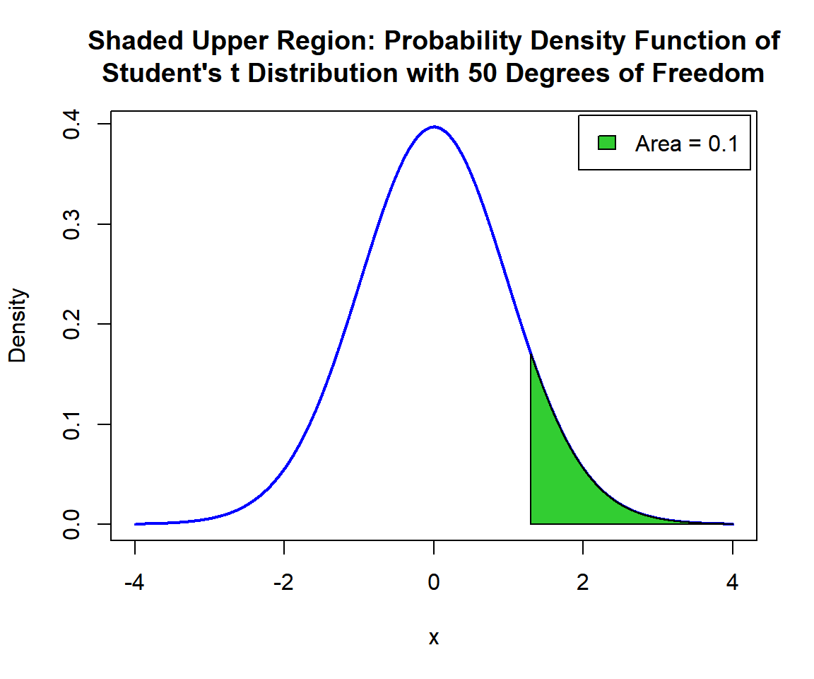
Shaded Upper Region: Probability Density Function (PDF) of Student’s t Distribution (50) in R
The feedback form is a Google form but it does not collect any personal information.
Please click on the link below to go to the Google form.
Thank You!
Go to Feedback Form
Copyright © 2020 - 2026. All Rights Reserved by Stats Codes