1 Test Statistic for Kruskal-Wallis Test in R
2 Simple Kruskal-Wallis Test in R
3 Kruskal-Wallis Test Critical Value in R
4 Kruskal-Wallis Test in R
5 Kruskal-Wallis Test: Test Statistics, P-value & Degrees of Freedom in R

Here, we discuss the Kruskal-Wallis test in R with interpretations, including, H-value, p-values, and critical values.

The Kruskal-Wallis test in R can be performed with the kruskal.test() function from the base "stats" package.

The Kruskal-Wallis test, with the assumption that the distributions have similar shapes or are symmetric, can be used to test whether the medians of the populations were two or more independent samples come from are equal (as stated in the null hypothesis) or not. It is a non-parametric alternative to the one-way ANOVA test, and a similar extension of the Wilcoxon rank-sum (Mann–Whitney U-test) to three or more groups.

In the Kruskal-Wallis test, the test statistic is based on the distribution of the ranks of each observation among all observations. It is the variance of average ranks between groups versus overall variance of ranks, and it follows a chi-squared distribution when the null hypothesis is true.

Kruskal-Wallis Tests & Hypotheses
Question	Are the group medians equal?
Null Hypothesis, $H_0$	$m_1 = m_2 = \dots = m_G$
Alternate Hypothesis, $H_1$	At least one group’s median is different from the rest

Sample Steps to Run a Kruskal-Wallis Test:

# Create the group data for the Kruskal-Wallis test
# Each row contains values for one group

x = c(5.9, 6.5, 7.0,
      8.0, 6.8, 7.3, 6.1, 7.3,
      6.0, 5.6, 5.8, 9.3)
groups = c("A", "A", "A",
           "B", "B", "B", "B", "B",
           "C", "C", "C", "C")

# Run the Kruskal-Wallis test with specifications

kruskal.test(x ~ groups)


    Kruskal-Wallis rank sum test

data:  x by groups
Kruskal-Wallis chi-squared = 2.4998, df = 2, p-value = 0.2865

Table of Some Kruskal-Wallis Tests Arguments in R
Argument	Usage
x ~ g	x contains the sample data values, g specifies the group they belong

Creating a Kruskal-Wallis Test Object:

# Create data
x = rnorm(60)
groups = rep(c("A", "B", "C"), each = 20)

# Create object
kwt_object = kruskal.test(x ~ groups)

# Extract a component
kwt_object$statistic

Kruskal-Wallis chi-squared 
                      0.26

Table of Some Kruskal-Wallis Test Object Outputs in R
Test Component	Usage
kwt_object$statistic	Test-statistic value
kwt_object$p.value	P-value
kwt_object$parameter	Degrees of freedom

1 Test Statistic for Kruskal-Wallis Test in R

The Kruskal-Wallis test has statistics, $H$, of the form:

\[\begin{align} H& =\frac{12}{N(N+1)} \sum_{j=1}^G \frac{r_{j\cdot}^2}{n_j} - 3(N+1) \\ & = \frac{12}{N(N+1)} \sum_{j=1}^G n_j \bar r_{j\cdot}^2 - 3(N+1).\end{align}\]

In cases where there are rank ties within groups, $H$ takes the form:

\[\begin{align} H& =\frac{\frac{12}{N(N+1)} \sum_{j=1}^G \frac{r_{j\cdot}^2}{n_j} - 3(N+1)}{1-\frac{\sum_{i=1}^T (t_i^3-t_i)}{N^3-N}} \\ & = \frac{\frac{12}{N(N+1)} \sum_{j=1}^G n_j \bar r_{j\cdot}^2 - 3(N+1)}{1-\frac{\sum_{i=1}^T (t_i^3-t_i)}{N^3-N}}.\end{align}\]

Inference on $H$ is based on the chi-squared distribution with $G - 1$ degrees of freedom.

$\text{rank}(3, 5, 5, 7, 9, 9, 9) = (1, 2.5, 2.5, 4, 6, 6, 6)$,

$G$ is the total number of groups,

$n_j$ is the number of observations from group $j$,

$N$ is the total number of observations, $\sum_{j=1}^G n_j$,

$r_{j\cdot}$ is the sum of the ranks for the observations from group $j$ among all the observations,

$\bar r_{j\cdot}$ is the average rank for the observations from group $j$ among all the observations,

$T$ is the number of sets of different tied ranks, and $t_i$ is the number of tied values for set $i$ that are tied at a particular value. $\frac{\sum_{i=1}^T (t_i^3-t_i)}{N^3-N}=0$ if there are no ties (all $t_i =1$).

2 Simple Kruskal-Wallis Test in R

Enter the data by hand.

x = c(17.8, 20.1, 20.6, 20.9, 19.1,
      17.9, 22.5, 19.3, 18.3, 19.5, 19.6,
      22.2, 20.2, 21.5, 19.0)
groups = c("A", "A", "A", "A", "A",
           "B", "B", "B", "B", "B", "B",
           "C", "C", "C", "C")

Using a boxplot, check variability between and within groups.

boxplot(x ~ groups,
     main = "X by Groups",
     xlab = "Groups",
     ylab = "X Value")

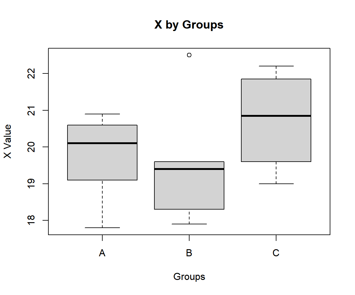
Simple Kruskal-Wallis Test Box Plot in R

The group sum of ranks, mean of ranks, and lengths; and overall lengths are:

xr = rank(x)
tapply(xr, groups, sum)

 A  B  C 
38 41 41

tapply(xr, groups, mean)

        A         B         C 
 7.600000  6.833333 10.250000

c(tapply(xr, groups, length), length(xr))

 A  B  C    
 5  6  4 15

For the following null hypothesis $H_0$, and alternative hypothesis $H_1$, with the level of significance $\alpha=0.05$.

$H_0:$ the group population medians are equal ($m_A = m_B = m_C$).

$H_1:$ at least one group’s median is different from the rest.

Because the level of significance is $\alpha=0.05$, the level of confidence is $1 - \alpha = 0.95$.

kruskal.test(x ~ groups)


    Kruskal-Wallis rank sum test

data:  x by groups
Kruskal-Wallis chi-squared = 1.4608, df = 2, p-value = 0.4817

The test statistic, $\chi^2$, is 1.4608,

the degrees of freedom are 2,

the p-value, $p$, is 0.4817.

Interpretation:

P-value: With the p-value ($p = 0.4817$) being greater than the level of significance 0.05, we fail to reject the null hypothesis that the group population medians are equal.
$\chi^2$ T-statistic: With test statistics value ($\chi^2_2 = 1.4608$) being less than the critical value, $\chi^2_{2, \alpha}=\text{qchisq(0.95, 2)}$$=5.9914645$ (or not in the shaded region), we fail to reject the null hypothesis that the group population medians are equal.

x = seq(0.01, 8, 1/1000); y = dchisq(x, df=2)
plot(x, y, type = "l",
     xlim = c(0, 8), ylim = c(-0.03, min(max(y), 1)),
     main = "Kruskal-Wallis Test
Shaded Region for Simple Test",
     xlab = "x", ylab = "Density",
     lwd = 2, col = "blue")
abline(h=0)
# Add shaded region and legend
point = qchisq(0.95, 2)
polygon(x = c(x[x >= point], 8, point),
        y = c(y[x >= point], 0, 0),
        col = "blue")
legend("topright", c("Area = 0.05"),
       fill = c("blue"), inset = 0.01)
# Add critical value and Chi-squared value
arrows(2.5, 0.4, 1.4608, 0)
text(2.5, 0.45, "Chi-squared = 1.4608")
text(5.991465, -0.02, expression(chi[G-1][','][alpha]^2==5.991465))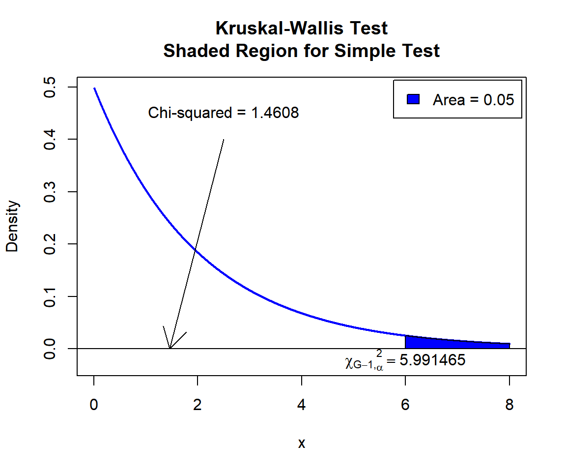

Kruskal-Wallis Test Shaded Region for Simple Test in R

3 Kruskal-Wallis Test Critical Value in R

To get the critical value for a Kruskal-Wallis test in R, you can use the qchisq() function for chi-squared distribution to derive the quantile associated with the given level of significance value $\alpha$.

The critical value is qchisq($1-\alpha$, df).

Example:

For $\alpha = 0.1$, and $\text{df} = 4$.

qchisq(0.9, 4)

[1] 7.77944

4 Kruskal-Wallis Test in R

Using the OrchardSprays data from the "datasets" package with 10 sample rows from 64 rows below:

OrchardSprays

   decrease rowpos colpos treatment
1        57      1      1         D
5        92      5      1         G
23       72      7      3         G
25      130      1      4         H
30       24      6      4         G
36        5      4      5         A
44       77      4      6         G
49        8      1      7         B
52       57      4      7         F
64       19      8      8         C

Using a boxplot, check variability between and within groups.

boxplot(decrease ~ treatment, data = OrchardSprays,
     main = "X by Groups",
     xlab = "Groups",
     ylab = "X Value")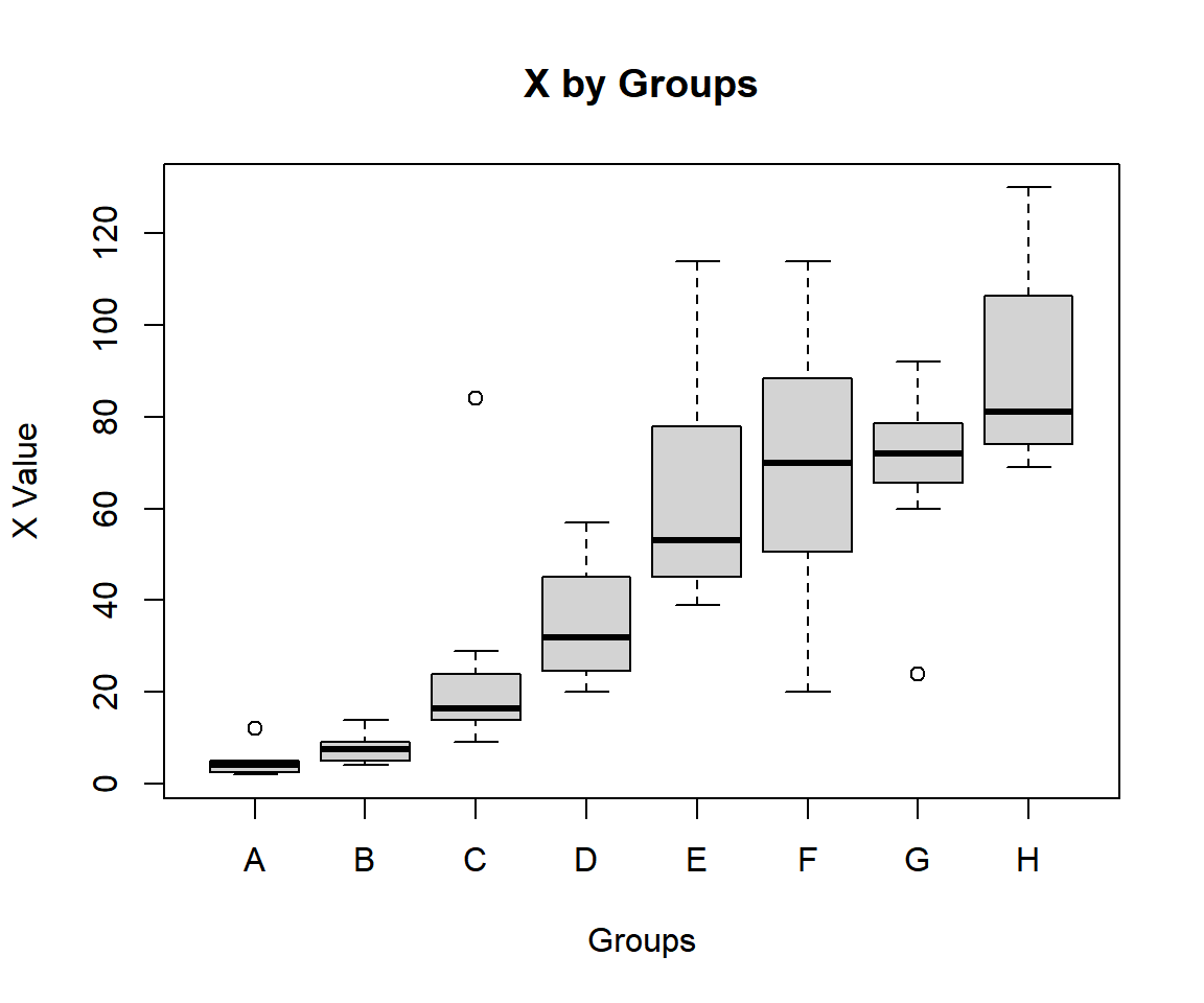

Kruskal-Wallis Test Box Plot in R

We consider decrease by treatment. The group sum of ranks, mean of ranks, and lengths; and overall lengths are:

xr = rank(OrchardSprays$decrease)
tapply(xr, OrchardSprays$treatment, sum)

    A     B     C     D     E     F     G     H 
 50.0  90.0 197.0 241.0 337.5 362.5 370.5 431.5

tapply(xr, OrchardSprays$treatment, mean)

      A       B       C       D       E       F       G       H 
 6.2500 11.2500 24.6250 30.1250 42.1875 45.3125 46.3125 53.9375

c(tapply(xr, OrchardSprays$treatment, length), length(xr))

 A  B  C  D  E  F  G  H    
 8  8  8  8  8  8  8  8 64

For the following null hypothesis $H_0$, and alternative hypothesis $H_1$, with the level of significance $\alpha=0.1$.

$H_0:$ the group population medians are equal ($m_A = m_B = \cdots = m_H$).

$H_1:$ at least one group’s median is different from the rest.

Because the level of significance is $\alpha=0.1$, the level of confidence is $1 - \alpha = 0.9$.

kruskal.test(decrease ~ treatment, data = OrchardSprays)


    Kruskal-Wallis rank sum test

data:  decrease by treatment
Kruskal-Wallis chi-squared = 48.874, df = 7, p-value = 2.402e-08

Interpretation:

P-value: With the p-value ($p = 2.402e-08$) being less than the level of significance 0.1, we reject the null hypothesis that the group population medians are equal.
$F$ T-statistic: With test statistics value ($\chi_7^2 = 48.874$) being in the critical region (shaded area), that is, $\chi_7^2 = 48.874$ greater than $\chi^2_{7, \alpha}=\text{qchisq(0.9, 7)}$$=12.0170366$, we reject the null hypothesis that the group population medians are equal.

x = seq(0.01, 50, 1/1000); y = dchisq(x, df=7)
plot(x, y, type = "l",
     xlim = c(0, 50), ylim = c(-0.008, min(max(y), 1)),
     main = "Kruskal-Wallis Test
Shaded Region",
     xlab = "x", ylab = "Density",
     lwd = 2, col = "blue")
abline(h=0)
# Add shaded region and legend
point = qchisq(0.9, 7)
polygon(x = c(x[x >= point], 50, point),
        y = c(y[x >= point], 0, 0),
        col = "blue")
legend("topright", c("Area = 0.1"),
       fill = c("blue"), inset = 0.01)
# Add critical value and Chi-squared value
arrows(35, 0.04, 48.874, 0)
text(35, 0.045, "Chi-squared = 48.874")
text(12.01704, -0.006, expression(chi[G-1][','][alpha]^2==12.01704))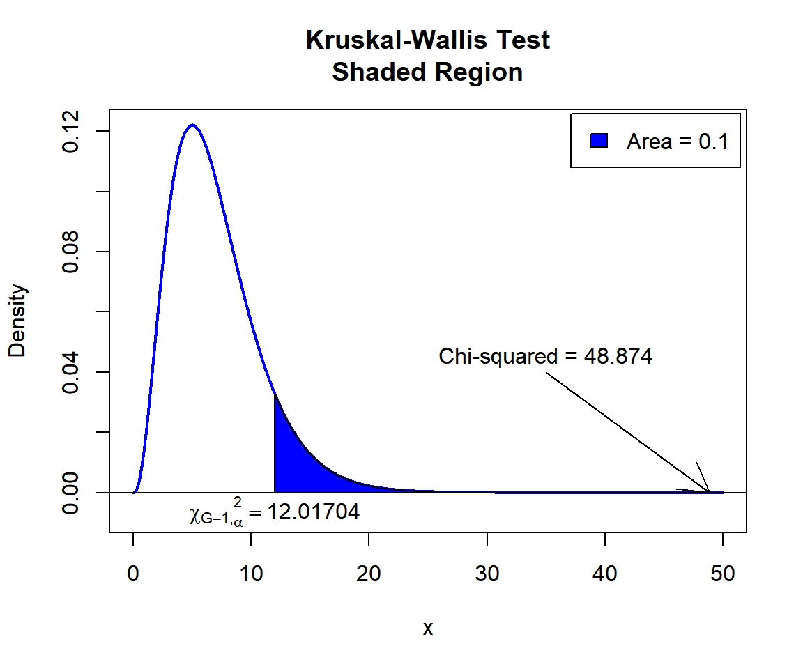

Kruskal-Wallis Test Shaded Region in R

5 Kruskal-Wallis Test: Test Statistics, P-value & Degrees of Freedom in R

Here for a Kruskal-Wallis test, we show how to get the test statistics (or H-value), p-values, and degrees of freedom from the kruskal.test() function in R, or by written code.

We consider count by spray.

kwt_object = kruskal.test(count ~ spray, data = InsectSprays)
kwt_object


    Kruskal-Wallis rank sum test

data:  count by spray
Kruskal-Wallis chi-squared = 54.691, df = 5, p-value = 1.511e-10

To get the test statistic (or H-value):

kwt_object$statistic

Kruskal-Wallis chi-squared 
                  54.69134

# to remove name "Kruskal-Wallis chi-squared"
unname(kwt_object$statistic)

[1] 54.69134

Same as:

#Method 1
x = InsectSprays$count
r = rank(x)
g = factor(InsectSprays$spray)
n = length(x)
ties = table(x)
scale_ranks = sum(tapply(r, g, "sum")^2 / tapply(r, g, "length"))
H = ((12 * scale_ranks / (n * (n + 1)) - 3 * (n + 1))/
      (1 - sum(ties^3 - ties) / (n^3 - n)))
H

[1] 54.69134

#Method 2
x = InsectSprays$count
r = rank(x)
g = factor(InsectSprays$spray)
n = length(x)
ties = table(x)
scale_ranks = sum(tapply(r, g, "mean")^2 * tapply(r, g, "length"))
H = ((12 * scale_ranks / (n * (n + 1)) - 3 * (n + 1))/
      (1 - sum(ties^3 - ties) / (n^3 - n)))
H

[1] 54.69134

To get the p-value:

The p-value is, $P \left(\chi^2_{df}> \text{observed} \right).$

kwt_object$p.value

[1] 1.510844e-10

Same as:

Note that the p-value depends on the $\text{test statistics}$ ($\chi^2_{df} = 54.69134$), and $\text{degrees of freedom}$ (5). We also use the distribution function pchisq() for the chi-squared distribution in R.

1-pchisq(54.69134, 5)

[1] 1.510848e-10

To get the degrees of freedom:

The degrees of freedom are $\text{df}=5$.

kwt_object$parameter

df 
 5

# to remove name df
unname(kwt_object$parameter)

[1] 5

Same as:

G = length(unique(g))
G-1

[1] 5

Question	Are the group medians equal?
Null Hypothesis, \(H_0\)	\(m_1 = m_2 = \dots = m_G\)
Alternate Hypothesis, \(H_1\)	At least one group’s median is different from the rest

Kruskal-Wallis Tests in R

Sample Steps to Run a Kruskal-Wallis Test:

Creating a Kruskal-Wallis Test Object:

1 Test Statistic for Kruskal-Wallis Test in R

2 Simple Kruskal-Wallis Test in R

Interpretation:

3 Kruskal-Wallis Test Critical Value in R

4 Kruskal-Wallis Test in R

Interpretation:

5 Kruskal-Wallis Test: Test Statistics, P-value & Degrees of Freedom in R

To get the test statistic (or H-value):

To get the p-value:

To get the degrees of freedom: