1 Test Statistic for Two Variances F-test in R
2 Simple Two Variances F-test in R
3 Two Variances F-test Critical Value in R
4 Two-tailed Two Variances F-test in R
5 One-tailed Two Variances F-test in R
6 Two Variances F-test: Test Statistics, P-value & Degree of Freedom in R
7 Two Variances F-test: Estimate & Confidence Interval in R

Here, we discuss the two variances F-test in R with interpretations, including, f-value, p-values, critical values, ratio of variances and confidence intervals.

The two variances F-test in R can be performed with the var.test() function from the base "stats" package.

The two variances F-test can be used to test whether the ratio of the variances of the populations where two independent random samples come from is equal to a certain value (stated in the null hypothesis) or not.

In the two variances F-test, the test statistic follows an F-distribution when the null hypothesis is true.

Two Variances F-tests & Hypotheses
Question	Are the variances equal, or ratio equal to $r_0$?	Is variance 1 greater than variance 2, or ratio greater than $r_0$?	Is variance 1 less than variance 2, or ratio less than $r_0$?
Form of Test	Two-tailed	Right-tailed test	Left-tailed test
Null Hypothesis, $H_0$	$\sigma^2_1/\sigma^2_2=1;$ $\quad$ $\sigma^2_1 / \sigma^2_2 = r_0$	$\sigma^2_1/\sigma^2_2=1;$ $\quad$ $\sigma^2_1 / \sigma^2_2 = r_0$	$\sigma^2_1/\sigma^2_2=1;$ $\quad$ $\sigma^2_1 / \sigma^2_2 = r_0$
Alternate Hypothesis, $H_1$	$\sigma^2_1/\sigma^2_2\neq1;$ $\quad$ $\sigma^2_1 / \sigma^2_2 \neq r_0$	$\sigma^2_1/\sigma^2_2>1;$ $\quad$ $\sigma^2_1 / \sigma^2_2 > r_0$	$\sigma^2_1/\sigma^2_2<1;$ $\quad$ $\sigma^2_1 / \sigma^2_2 < r_0$

Sample Steps to Run a Two Variances F-test:

# Create the data samples for the two variances F-test

data1 = c(12.9, 9.9, 10.5, 10.6, 10.4)
data2 =  c(9.8, 12.4, 12.6, 7.6,
           11.0, 9.1, 8.0, 12.4)

# Run the two variances F-test with specifications

var.test(data1, data2, ratio = 1,
         alternative = "two.sided",
         conf.level = 0.95)


    F test to compare two variances

data:  data1 and data2
F = 0.33327, num df = 4, denom df = 7, p-value = 0.3051
alternative hypothesis: true ratio of variances is not equal to 1
95 percent confidence interval:
 0.06034607 3.02411060
sample estimates:
ratio of variances 
         0.3332669

Table of Some Two Variances F-tests Arguments in R
Argument	Usage
x, y	The two sample data values
x ~ y	x contains the two sample data values, y specifies the group they belong
ratio	The value of the ratio in the null hypothesis
alternative	Set alternate hypothesis as "greater", "less", or the default "two.sided"
conf.level	Level of confidence for the test and confidence interval (default = 0.95)

Creating a Two Variances F-test Object:

# Create data
data1 = rnorm(100); data2 = rnorm(200)

# Create object
var_object = var.test(data1, data2, ratio = 1,
                      alternative = "two.sided",
                      conf.level = 0.95)

# Extract a component
var_object$statistic

        F 
0.7466371

Table of Some Two Variances F-test Object Outputs in R
Test Component	Usage
var_object$statistic	Test-statistic value
var_object$p.value	P-value
var_object$parameter	Degrees of freedom
var_object$estimate	Point estimate or sample ratio of variances
var_object$conf.int	Confidence interval

1 Test Statistic for Two Variances F-test in R

The two variances F-test has test statistics, $F$, of the form:

when $\sigma^2_1=\sigma^2_2$ or $\sigma^2_1/\sigma^2_2=1,$

\[F = \frac{s^2_1}{s^2_2};\]

when $\sigma^2_1/\sigma^2_2 = r_0,$

\[F = \frac{s^2_1/\sigma^2_1}{s^2_2/\sigma^2_2} = \frac{s^2_1}{s^2_2}\frac{\sigma^2_2}{\sigma^2_1} = \frac{s^2_1}{s^2_2}\frac{1}{r_0}.\]

For independent random samples that come from normal distributions, $F$ is said to follow the F-distribution $\left(F_{n_1-1,n_2-1}\right)$ when the null hypothesis is true, with $n_1 - 1$ numerator degrees of freedom, and $n_2 - 1$ denominator degrees of freedom.

$s^2_1$ and $s^2_2$ are the sample variances of $\text{group 1}$ and $\text{group 2}$ respectively,

$\sigma^2_1$ and $\sigma^2_2$ are the population variances of $\text{group 1}$ and $\text{group 2}$ respectively,

$n_1$ and $n_2$ are the number of observations in $\text{group 1}$ and $\text{group 2}$ respectively,

and $r_0$ is the value of the ratio $(\sigma_1^2/\sigma_2^2)$ to be tested and set in the null hypothesis.

2 Simple Two Variances F-test in R

Enter the data by hand.

data1 = c(13.0, 10.0, 10.8, 8.4, 8.8,
          9.8, 6.3, 8.2, 6.1, 3.6,
          11.0, 8.7)
data2 = c(49.0, 48.9, 47.5, 49.8, 51.9,
          49.3, 50.4, 53.0, 52.4, 48.3,
          48.1, 51.3, 53.0, 53.3, 48.7)

The sample variances are $s^2_1 = 6.3602273$ (var(data1)), and $s^2_2 = 3.9778095$ (var(data2)).

For the following null hypothesis $H_0$, and alternative hypothesis $H_1$, with the level of significance $\alpha=0.05$.

$H_0:$ the two population variances are equal ($\sigma^2_1/\sigma^2_2=1$).

$H_1:$ the two population variances are not equal ($\sigma^2_1/\sigma^2_2\neq1$, hence the default two-sided).

Because the level of significance is $\alpha=0.05$, the level of confidence is $1 - \alpha = 0.95$.

The var.test() function has the default ratio as 1, the default alternative as "two.sided", and the default level of confidence as 0.95, hence, you do not need to specify the "ratio", "alternative", and "conf.level" arguments in this case.

var.test(data1, data2, ratio = 1,
         alternative = "two.sided", 
         conf.level = 0.95)

Or:

var.test(data1, data2)


    F test to compare two variances

data:  data1 and data2
F = 1.5989, num df = 11, denom df = 14, p-value = 0.4041
alternative hypothesis: true ratio of variances is not equal to 1
95 percent confidence interval:
 0.5166847 5.3704925
sample estimates:
ratio of variances 
          1.598927

The ratio of variances, the test statistic, $F$, is 1.5989,

the degrees of freedom, are numerator df $n_1-1= 11$, denominator df $n_2-1= 14$,

the p-value, $p$, is 0.4041,

the 95% confidence interval is [0.5166847, 5.3704925].

Interpretation:

P-value: With the p-value ($p = 0.4041$) being greater than the level of significance 0.05, we fail to reject the null hypothesis that the ratio of variances is equal to 1.
$F$ T-statistic: With test statistics value ($F_{11, 14} = 1.5989$) being between the critical values, $F_{11, 14, \alpha/2}=\text{qf(0.025, 11, 14)}$$=0.2977245$ and $F_{11, 14, 1-\alpha/2}=\text{qf(0.975, 11, 14)}$$=3.0945898$ (or not in the shaded region), we fail to reject the null hypothesis that the ratio of variances is equal to 1.
Confidence Interval: With the null hypothesis ratio of variances ($\sigma^2_1 / \sigma^2_2 = 1$) being inside the confidence interval, $[0.5166847, 5.3704925]$, we fail to reject the null hypothesis that the ratio of variances is equal to 1.

x = seq(0.01, 5, 1/1000); y = df(x, df1=11, df2=14)
plot(x, y, type = "l",
     xlim = c(0, 5), ylim = c(-0.06, min(max(y), 1)),
     main = "Two Variances F-test
Shaded Region for Simple Test",
     xlab = "x", ylab = "Density",
     lwd = 2, col = "blue")
abline(h=0)
# Add shaded region and legend
point1 = qf(0.025, 11, 14); point2 = qf(0.975, 11, 14)
polygon(x = c(0, x[x <= point1], point1),
        y = c(0, y[x <= point1], 0),
        col = "blue")
polygon(x = c(x[x >= point2], 5, point2),
        y = c(y[x >= point2], 0, 0),
        col = "blue")
legend("topright", c("Area = 0.05"),
       fill = c("blue"), inset = 0.01)
# Add critical value and F-value
arrows(2.5, 0.4, 1.5989, 0)
text(2.5, 0.45, "F = 1.5989")
text(0.2977+0.1, -0.04, expression(F[alpha/2]==0.2977))
text(3.09459, -0.04, expression(F[1-alpha/2]==3.09459))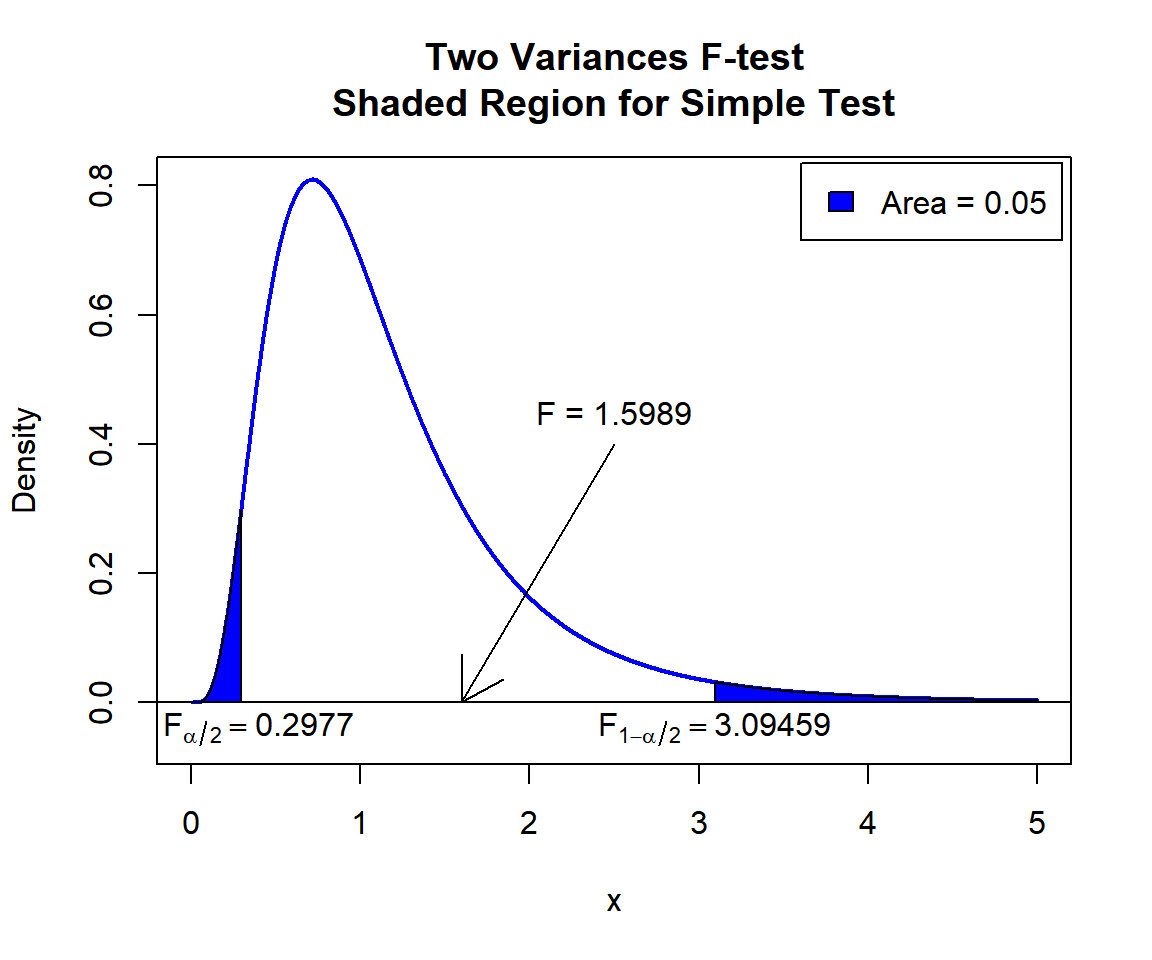

Two Variances F-test Shaded Region for Simple Test in R

See line charts, shading areas under a curve, lines & arrows on plots, mathematical expressions on plots, and legends on plots for more details on making the plot above.

3 Two Variances F-test Critical Value in R

To get the critical value for a two variances F-test in R, you can use the qf() function for F-distribution to derive the quantile associated with the given level of significance value $\alpha$.

For two-tailed test with level of significance $\alpha$. The critical values are: qf($\alpha/2$, df1, df2) and qf($1-\alpha/2$, df1, df2).

For one-tailed test with level of significance $\alpha$. The critical value is: for left-tailed, qf($\alpha$, df1, df2); and for right-tailed, qf($1-\alpha$, df1, df2).

Example:

For $\alpha = 0.1$, $\text{df1} = 15$, and $\text{df2} = 25$.

Two-tailed:

qf(0.05, 15, 25); qf(0.95, 15, 25)

[1] 0.4386486

[1] 2.088887

One-tailed:

#Left
qf(0.1, 15, 25)

[1] 0.5280184

#Right
qf(0.9, 15, 25)

[1] 1.770834

4 Two-tailed Two Variances F-test in R

Using the warpbreaks data from the "datasets" package with 10 sample rows from 54 rows below:

warpbreaks

   breaks wool tension
1      26    A       L
5      70    A       L
19     36    A       H
23     10    A       H
25     28    A       H
30     29    B       L
36     44    B       L
44     39    B       M
49     17    B       H
54     28    B       H

For Wool type A as group 1 versus Wool type B as group 2.

The sample variances are $s^2_1 = 251.2678063$ and $s^2_2 = 86.5071225$.

tapply(warpbreaks$breaks, warpbreaks$wool, var)

        A         B 
251.26781  86.50712

For the following null hypothesis $H_0$, and alternative hypothesis $H_1$, with the level of significance $\alpha=0.1$.

$H_0:$ the ratio of population variances is equal to 1.4 ($\sigma^2_1 / \sigma^2_2 = 1.4$).

$H_1:$ the ratio of population variances is not equal to 1.4 ($\sigma^2_1 / \sigma^2_2 \neq 1.4$, hence the default two-sided).

Because the level of significance is $\alpha=0.1$, the level of confidence is $1 - \alpha = 0.9$.

# This example uses var.test(x ~ y). For var.test(x, y), see other examples above or below.
var.test(breaks ~ wool, data = warpbreaks, 
         ratio = 1.4,
         alternative = "two.sided", 
         conf.level = 0.9)


    F test to compare two variances

data:  breaks by wool
F = 2.0747, num df = 26, denom df = 26, p-value = 0.06827
alternative hypothesis: true ratio of variances is not equal to 1.4
90 percent confidence interval:
 1.505584 5.603574
sample estimates:
ratio of variances 
          2.904591

Interpretation:

P-value: With the p-value ($p = 0.06827$) being less than the level of significance 0.1, we reject the null hypothesis that the ratio of variances is equal to 1.4.
$F$ T-statistic: With test statistics value ($F_{26, 26} = 2.0747$) being in the critical region (shaded area), that is, $F_{26, 26} = 2.0747$ greater than $F_{26, 26, 1-\alpha/2}=\text{qf(0.95, 26, 26)}$$=1.9292127$, we reject the null hypothesis that the ratio of variances is equal to 1.4.
Confidence Interval: With the null hypothesis ratio of variances ($\sigma^2_1 / \sigma^2_2 = 1.4$) being outside the confidence interval, $[1.505584, 5.603574]$, we reject the null hypothesis that the ratio of variances is equal to 1.4.

x = seq(0.01, 4, 1/1000); y = df(x, df1=26, df2=26)
plot(x, y, type = "l",
     xlim = c(0, 4), ylim = c(-0.06, max(y)),
     main = "Two Variances F-test
Shaded Region for Two-tailed Test",
     xlab = "x", ylab = "Density",
     lwd = 2, col = "blue")
abline(h=0)
# Add shaded region and legend
point1 = qf(0.05, 26, 26); point2 = qf(0.95, 26, 26)
polygon(x = c(0, x[x <= point1], point1),
        y = c(0, y[x <= point1], 0),
        col = "blue")
polygon(x = c(x[x >= point2], 4, point2),
        y = c(y[x >= point2], 0, 0),
        col = "blue")
legend("topright", c("Area = 0.1"),
       fill = c("blue"), inset = 0.01)
# Add critical value and F-value
arrows(2.0747, 0.3, 2.0747, 0)
text(2.0747, 0.35, expression(F==2.0747))
text(0.5183462, -0.04, expression(F[alpha/2]==0.5183462))
text(1.929213, -0.04, expression(F[1-alpha/2]==1.929213))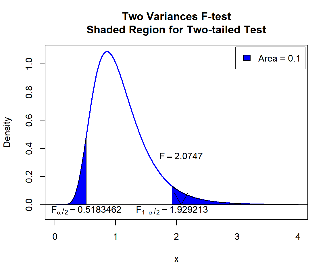

Two Variances F-test Shaded Region for Two-tailed Test in R

5 One-tailed Two Variances F-test in R

Right Tailed Test

Using the stackloss data from the "datasets" package with 10 sample rows from 21 below:

stackloss

   Air.Flow Water.Temp Acid.Conc. stack.loss
1        80         27         89         42
3        75         25         90         37
4        62         24         87         28
6        62         23         87         18
7        62         24         93         19
11       58         18         89         14
12       58         17         88         13
15       50         18         89          8
16       50         18         86          7
21       70         20         91         15

For “Air.Flow” as group 1 versus “Acid.Conc.” as group 2.

The sample variances are $s^2_1 = 84.0571429$ (var(stackloss$Air.Flow)), and $s^2_2 = 28.7142857$ (var(stackloss$Acid.Conc.)).

For the following null hypothesis $H_0$, and alternative hypothesis $H_1$, with the level of significance $\alpha=0.2$.

$H_0:$ the two population variances are equal ($\sigma^2_1/\sigma^2_2=1$).

$H_1:$ the variance of population 1 is greater than the variance of population 2 ($\sigma^2_1/\sigma^2_2>1$, hence one-sided).

Because the level of significance is $\alpha=0.2$, the level of confidence is $1 - \alpha = 0.8$.

var.test(stackloss$Air.Flow, stackloss$Acid.Conc.,
         ratio = 1,
         alternative = "greater",
         conf.level = 0.8)


    F test to compare two variances

data:  stackloss$Air.Flow and stackloss$Acid.Conc.
F = 2.9274, num df = 20, denom df = 20, p-value = 0.0102
alternative hypothesis: true ratio of variances is greater than 1
80 percent confidence interval:
 1.997399      Inf
sample estimates:
ratio of variances 
          2.927363

Interpretation:

P-value: With the p-value ($p = 0.0102$) being less than the level of significance 0.2, we reject the null hypothesis that the ratio of variances is equal to 1.
$F$ T-statistic: With test statistics value ($F_{20, 20} = 2.9274$) being greater than the critical value, $F_{20, 20, 1-\alpha}=\text{qf(0.8, 20, 20)}$$=1.4655876$ (or in the shaded region), we reject the null hypothesis that the ratio of variances is equal to 1.
Confidence Interval: With the null hypothesis ratio of variances value ($\sigma^2_1 / \sigma^2_2 = 1$) being outside the confidence interval, $[1.997399,\infty)$, we reject the null hypothesis that the ratio of variances is equal to 1.

plot(x, y, type = "l",
     xlim = c(0, 4), ylim = c(-0.06, max(y)),
     main = "Two Variances F-test
Shaded Region for Right-tailed Test",
     xlab = "x", ylab = "Density",
     lwd = 2, col = "blue")
abline(h=0)
# Add shaded region and legend
point = qf(0.8, 20, 20)
polygon(x = c(x[x >= point], 4, point),
        y = c(y[x >= point], 0, 0),
        col = "blue")
legend("topright", c("Area = 0.2"),
       fill = c("blue"), inset = 0.01)
# Add critical value and F-value
arrows(2.9274, 0.3, 2.9274, 0)
text(2.9274, 0.35, expression(F==2.9274))
text(1.465588, -0.04, expression(F[1-alpha]==1.465588))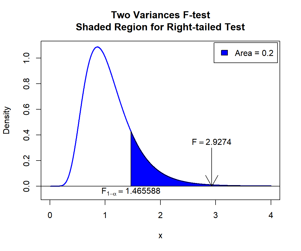

Two Variances F-test Shaded Region for Right-tailed Test in R

Left Tailed Test

For “Acid.Conc.” as group 1 versus “Air.Flow” as group 2.

The sample variances are $s^2_1 = 28.7142857$ (var(stackloss$Acid.Conc.)), and $s^2_2 = 84.0571429$ (var(stackloss$Air.Flow)).

For the following null hypothesis $H_0$, and alternative hypothesis $H_1$, with the level of significance $\alpha=0.1$.

$H_0:$ the ratio of population variances is equal to 0.5 ($\sigma^2_1 / \sigma^2_2 = 0.5$).

$H_1:$ the ratio of population variances is less than 0.5 ($\sigma^2_1 / \sigma^2_2 < 0.5$, hence one-sided).

Because the level of significance is $\alpha=0.1$, the level of confidence is $1 - \alpha = 0.9$.

var.test(stackloss$Acid.Conc., stackloss$Air.Flow,
         ratio  = 0.5,
         alternative = "less",
         conf.level = 0.9)


    F test to compare two variances

data:  stackloss$Acid.Conc. and stackloss$Air.Flow
F = 0.68321, num df = 20, denom df = 20, p-value = 0.2008
alternative hypothesis: true ratio of variances is less than 0.5
90 percent confidence interval:
 0.0000000 0.6127847
sample estimates:
ratio of variances 
         0.3416044

Interpretation:

P-value: With the p-value ($p = 0.2008$) being greater than the level of significance 0.1, we fail to reject the null hypothesis that the ratio of variances is equal to 0.5.
$F$ T-statistic: With test statistics value ($F_{20, 20} = 0.68321$) being greater than the critical value, $F_{20, 20, \alpha}=\text{qf(0.1, 20, 20)}$$=0.5574623$ (or not in the shaded region), we fail to reject the null hypothesis that the ratio of variances is equal to 0.5.
Confidence Interval: With the null hypothesis ratio of variances value ($\sigma^2_1 / \sigma^2_2 = 0.5$) being inside the confidence interval, $(0, 0.6127847]$, we fail reject the null hypothesis that the ratio of variances is equal to 0.5.

plot(x, y, type = "l",
     xlim = c(0, 4), ylim = c(-0.06, max(y)),
     main = "Two Variances F-test
Shaded Region for Left-tailed Test",
     xlab = "x", ylab = "Density",
     lwd = 2, col = "blue")
abline(h=0)
# Add shaded region and legend
point = qf(0.1, 20, 20)
polygon(x = c(0, x[x <= point], point),
        y = c(0, y[x <= point], 0),
        col = "blue")
legend("topright", c("Area = 0.1"),
       fill = c("blue"), inset = 0.01)
# Add critical value and F-value
arrows(1, 0.3, 0.68321, 0)
text(1, 0.35, expression(F==0.68321))
text(0.5574623, -0.04, expression(F[alpha]==0.5574623))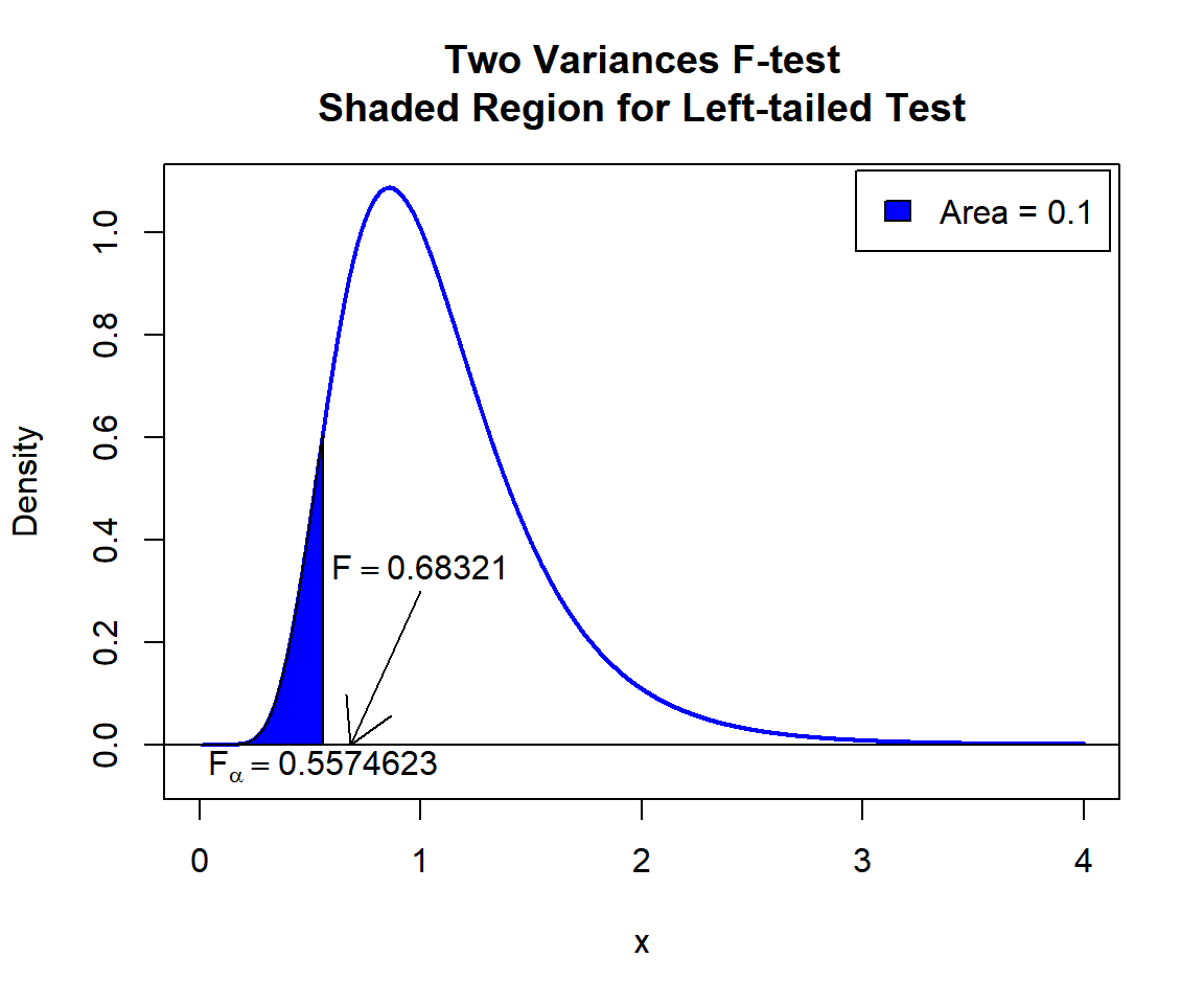

Two Variances F-test Shaded Region for Left-tailed Test in R

6 Two Variances F-test: Test Statistics, P-value & Degree of Freedom in R

Here for a two variances F-test, we show how to get the test statistics (or f-value), p-values, and degrees of freedom from the var.test() function in R, or by written code.

data1 = stackloss$Air.Flow; data2 = stackloss$Acid.Conc.
var_object = var.test(data1, data2, ratio = 2,
                      alternative = "two.sided",
                      conf.level = 0.95)
var_object


    F test to compare two variances

data:  data1 and data2
F = 1.4637, num df = 20, denom df = 20, p-value = 0.4016
alternative hypothesis: true ratio of variances is not equal to 2
95 percent confidence interval:
 1.187820 7.214441
sample estimates:
ratio of variances 
          2.927363

To get the test statistic or f-value:

\[F = \frac{s^2_1/\sigma^2_1}{s^2_2/\sigma^2_2} = \frac{s^2_1}{s^2_2}\frac{\sigma^2_2}{\sigma^2_1} = \frac{s^2_1}{s^2_2}\frac{1}{r_0}.\]

var_object$statistic

       F 
1.463682

# to remove name F
unname(var_object$statistic)

[1] 1.463682

Same as:

s1 = var(data1)
s2 = var(data2)
ratio = 2
(s1/s2)*(1/ratio)

[1] 1.463682

To get the p-value:

Two-tailed: For test statistics, $F_{Observed}$.

$Pvalue$ is the smaller of $2*P(F_{df1, df2}>F_{Observed})$ or $2*P(F_{df1, df2}<F_{Observed})$.

One-tailed: For right-tail, $Pvalue = P(F_{df1, df2}>F_{Observed})$ or for left-tail, $Pvalue = P(F_{df1, df2}<F_{Observed})$.

var_object$p.value

[1] 0.4015967

Same as:

Note that the p-value depends on the $\text{test statistics}$ ($F_{df1, df2} = 1.4637$), and $\text{degrees of freedom}$ (20, 20). We also use the distribution function pf() for the F distribution in R.

2*(1-pf(1.463682, 20, 20))

[1] 0.4015964

min(2*(1-pf(1.463682, 20, 20)), 2*pf(1.463682, 20, 20))

[1] 0.4015964

To get the degrees of freedom:

The degrees of freedom are $\text{df1}=20$ and $\text{df2}=20$.

var_object$parameter

  num df denom df 
      20       20

# to remove names num df, denom df
unname(var_object$parameter)

[1] 20 20

Same as:

length(data1)-1; length(data2)-1

[1] 20

[1] 20

7 Two Variances F-test: Estimate & Confidence Interval in R

Here for a two variances F-test, we show how to get the ratio of variances and confidence interval from the var.test() function in R, or by written code.

data1 = stackloss$Air.Flow; data2 = stackloss$Acid.Conc.
var_object = var.test(data1, data2, ratio = 2,
                      alternative = "two.sided", 
                      conf.level = 0.9)
var_object


    F test to compare two variances

data:  data1 and data2
F = 1.4637, num df = 20, denom df = 20, p-value = 0.4016
alternative hypothesis: true ratio of variances is not equal to 2
90 percent confidence interval:
 1.378131 6.218174
sample estimates:
ratio of variances 
          2.927363

To get the point estimate or ratio of variances:

\[r = \frac{s^2_1}{s^2_2}.\]

var_object$estimate

ratio of variances 
          2.927363

# to remove name ratio of variances
unname(var_object$estimate)

[1] 2.927363

Same as:

sv1 = var(data1); sv2 = var(data2)
sv1/sv2

[1] 2.927363

To get the confidence interval for $\sigma_1^2 / \sigma_2^2$:

For two-tailed:

\[CI = \left[\frac{s^2_1/s^2_2}{F_{df1, df2, 1-\alpha/2}} \;,\; \frac{s^2_1/s^2_2}{F_{df1, df2, \alpha/2}} \right].\]

For right one-tailed:

\[CI = \left[\frac{s^2_1/s^2_2}{F_{df1, df2, 1-\alpha}} \;,\; \infty \right).\]

For left one-tailed:

\[CI = \left(0 \;,\; \frac{s^2_1/s^2_2}{F_{df1, df2, \alpha}} \right].\]

var_object$conf.int

[1] 1.378131 6.218174
attr(,"conf.level")
[1] 0.9

# to remove attr conf.int
var_object$conf.int[1:2]

[1] 1.378131 6.218174

Same as:

s1 = var(data1); s2 = var(data2)
alpha = 0.1
fl = qf(1-alpha/2, 20, 20)
l = (s1/s2)*(1/fl)
fu = qf(alpha/2, 20, 20)
u = (s1/s2)*(1/fu)
c(l, u)

[1] 1.378131 6.218174

One tailed example:

s1 = var(data1); s2 = var(data2)
alpha = 0.1
# Right Tail
fl = qf(1-alpha, 20, 20)
l = (s1/s2)*(1/fl)
c(l, Inf)
# Left Tail
fu = qf(alpha, 20, 20)
u = (s1/s2)*(1/fu)
c(0, u)

Question	Are the variances equal, or ratio equal to \(r_0\)?	Is variance 1 greater than variance 2, or ratio greater than \(r_0\)?	Is variance 1 less than variance 2, or ratio less than \(r_0\)?
Form of Test	Two-tailed	Right-tailed test	Left-tailed test
Null Hypothesis, \(H_0\)	\(\sigma^2_1/\sigma^2_2=1;\) \(\quad\) \(\sigma^2_1 / \sigma^2_2 = r_0\)	\(\sigma^2_1/\sigma^2_2=1;\) \(\quad\) \(\sigma^2_1 / \sigma^2_2 = r_0\)	\(\sigma^2_1/\sigma^2_2=1;\) \(\quad\) \(\sigma^2_1 / \sigma^2_2 = r_0\)
Alternate Hypothesis, \(H_1\)	\(\sigma^2_1/\sigma^2_2\neq1;\) \(\quad\) \(\sigma^2_1 / \sigma^2_2 \neq r_0\)	\(\sigma^2_1/\sigma^2_2>1;\) \(\quad\) \(\sigma^2_1 / \sigma^2_2 > r_0\)	\(\sigma^2_1/\sigma^2_2<1;\) \(\quad\) \(\sigma^2_1 / \sigma^2_2 < r_0\)

Two Variances F-tests in R

Sample Steps to Run a Two Variances F-test:

Creating a Two Variances F-test Object:

1 Test Statistic for Two Variances F-test in R

2 Simple Two Variances F-test in R

Interpretation:

3 Two Variances F-test Critical Value in R

4 Two-tailed Two Variances F-test in R

Interpretation:

5 One-tailed Two Variances F-test in R

Right Tailed Test

Interpretation:

Left Tailed Test

Interpretation:

6 Two Variances F-test: Test Statistics, P-value & Degree of Freedom in R

To get the test statistic or f-value:

To get the p-value:

To get the degrees of freedom:

7 Two Variances F-test: Estimate & Confidence Interval in R

To get the point estimate or ratio of variances:

To get the confidence interval for \(\sigma_1^2 / \sigma_2^2\):