Two Proportions Tests (with Z & Chi-squared) in R
- 1 Test Statistic for Two Proportions Test in R
- 2 Simple Two Proportions Test in R
- 3 Two Proportions Test Critical Value in R
- 4 Two-tailed Two Proportions Test in R
- 5 One-tailed Two Proportions Test in R
- 6 Two Proportions Test with Known Null Proportions in R
- 7 Two Proportions Test: Test Statistics, P-value & Degree of Freedom in R
- 8 Two Proportions Test: Estimates & Confidence Interval in R
Here, we discuss the two proportions tests in R with interpretations, including, chi-squared value, p-values, critical values, and confidence intervals.
The two proportions test in R can be performed with the
prop.test() function from the base "stats" package.
The two proportions test can be used to test whether the proportions of successes in the populations where two independent random samples come from are equal (as stated in the null hypothesis) or not.
In the two proportions test, the test statistic follows a chi-squared distribution with 1 degree of freedom (or standard normal distribution) when the null hypothesis is true.
| Question | Are the proportions equal? | Is proportion 1 greater than proportion 2? | Is proportion 1 less than proportion 2? |
| Form of Test | Two-tailed | Right-tailed test | Left-tailed test |
| Null Hypothesis, \(H_0\) | \(p_1 = p_2\) | \(p_1 = p_2\) | \(p_1 = p_2\) |
| Alternate Hypothesis, \(H_1\) | \(p_1 \neq p_2\) | \(p_1 > p_2\) | \(p_1 < p_2\) |
Sample Steps to Run a Two Proportions Test:
# Specify:
# x1 & x2 as the number of successes
# n1 & n2 as the number of trials

# Run the two proportion test with specifications

prop.test(c(x1 = 45, x2 = 65), c(n1 = 100, n2 = 120),
          alternative = "two.sided",
          conf.level = 0.95, correct = FALSE)
    2-sample test for equality of proportions without continuity correction

data:  c(x1 = 45, x2 = 65) out of c(n1 = 100, n2 = 120)
X-squared = 1.8333, df = 1, p-value = 0.1757
alternative hypothesis: two.sided
95 percent confidence interval:
 -0.22378432  0.04045098
sample estimates:
   prop 1    prop 2
0.4500000 0.5416667 | Argument | Usage |
| x | Sample count of number of successes as a vector |
| n | Sample count of number of trials as a vector |
| alternative | Set alternate hypothesis as "greater", "less", or the default "two.sided" |
| conf.level | Level of confidence for the test and confidence interval (default = 0.95) |
| correct | Set to FALSE to remove continuity correction (default =
TRUE) |
Creating a Two Proportions Test Object:
# Create object with:
# x1 & x2 as the number of successes
# n1 & n2 as the number of trials
prop_object = prop.test(c(x1 = 45, x2 = 65), c(n1 = 100, n2 = 120),
                        alternative = "two.sided",
                        conf.level = 0.95, correct = FALSE)

# Extract a component
prop_object$statistic
X-squared
1.833333 | Test Component | Usage |
| prop_object$statistic | Test-statistic value |
| prop_object$p.value | P-value |
| prop_object$parameter | Degrees of freedom |
| prop_object$estimate | Point estimates or sample proportions |
| prop_object$conf.int | Confidence interval |
1 Test Statistic for Two Proportions Test in R
For \(\chi^2_1\), which is the
chi-squared distribution with 1 degree of freedom, and \(z\), which is the standard normal
distribution (mean is 0, and standard
deviation is 1), the two proportions test has test statistics, \(\chi^2_1\) (or \(z^2\)), without continuity correction
(correct = FALSE), which takes the form:
\[z = \frac{(\frac{x_1}{n_1}-\frac{x_2}{n_2})}{\sqrt {\hat p(1-\hat p) \left(\frac{1}{n_1} + \frac{1}{n_2} \right)}} \quad \text{or} \quad \chi^2_1=\sum_{i,j=1}^{2}\frac{(O_{ij}-E_{ij})^2}{E_{ij}},\]
where
\[\hat p = \frac{x_1 + x_2}{n_1 + n_2}.\]
In cases where Yates’ continuity correction is applied (default in R), it takes the form:
\[z = \frac{(\frac{x_1 \pm c}{n_1}-\frac{x_2 \pm c}{n_2})}{\sqrt {\hat p(1-\hat p) \left(\frac{1}{n_1} + \frac{1}{n_2} \right)}} \quad \text{or} \quad \chi^2_1=\sum_{i,j=1}^{2}\frac{(|O_{ij}-E_{ij}|-c)^2}{E_{ij}}.\] Note that \(z^2 = \chi^2_1\) in both cases. However, for one-sided tests, the level of significance \(\alpha\) for \(z\) is \(2\alpha\) for \(\chi^2_1\).
| \(z\) test | \(\chi^2_1\) test |
|---|---|
| \(x_1\) and \(x_2\) are the number of successes, \(n_1\) and \(n_2\) are the number of trials | \(O_{ij}'s\) are the observed values (\(O_{11} = x_1\), \(O_{21} = x_2\), \(O_{12} = n_1-x_1\), and \(O_{22} = n_2-x_2\)) |
| \(\hat p\) is the pooled sample proportion value | \(E_{ij}'s\) are the expected values (\(E_{11} = n_1\hat p\), \(E_{21} = n_2\hat p\), \(E_{12} = n_1(1-\hat p)\), and \(E_{22} = n_2(1-\hat p)\)) |
|
\(c = \min\{0.5, k\}\), with \(k = |n_2x_1-n_1x_2|/(n_1+n_2)\) For \(i = \{1, 2\}\), \(x_i+c \;\) when \(n_i \hat p \geq x_i\), and \(x_i-c \;\) when \(n_i \hat p < x_i\) |
\(c = \min\{0.5, k\}\), with \(k = |n_2x_1-n_1x_2|/(n_1+n_2)\) |
The test is ideal for large samples sizes (for example, each
\(n_ip_i > 5\) \(\&\) \(n_i(1-p_i) > 5\)).
See also the one proportion test.
2 Simple Two Proportions Test in R
With number of successes, \(x_1 = 62\) and \(x_2 = 44\), in \(n_1 = 120\) and \(n_2 = 100\) trials.
For the following null hypothesis \(H_0\), and alternative hypothesis \(H_1\), with the level of significance \(\alpha=0.05\), applying continuity correction.
\(H_0:\) the difference in population proportions is equal to 0 (\(p_1 - p_2 = 0\)).
\(H_1:\) the difference in population proportions is not equal to 0 (\(p_1 - p_2 \neq 0\), hence the default two-sided).
Because the level of significance is \(\alpha=0.05\), the level of confidence is \(1 - \alpha = 0.95\).
The prop.test() function has the default
alternative as "two.sided", the default level of
confidence as 0.95, and the default method as
continuity corrected, hence, you do not need to specify the
"alternative", "conf.level" and "correct" arguments in this
case.
Or:
    2-sample test for equality of proportions with continuity correction

data:  c(62, 44) out of c(120, 100)
X-squared = 0.99541, df = 1, p-value = 0.3184
alternative hypothesis: two.sided
95 percent confidence interval:
 -0.06463441  0.21796774
sample estimates:
   prop 1    prop 2
0.5166667 0.4400000
The sample proportions are, \(\hat p_1 = x_1/n_1\), is 0.5166667, and \(\hat p_2 = x_2/n_2\), is 0.44,
test statistic, \(\chi^2_1\), is 0.99541,
the degree of freedom is 1,
the p-value, \(p\), is 0.3184,
the 95% confidence interval is [-0.06463441, 0.21796774].
Interpretation:
Note that for prop.test() in R, the two proportions
test’s p-value and T-statistic methods may disagree with the confidence
interval method for some edge cases. This is because the p-value and
T-statistic are based on pooled standard
error estimate, while the confidence interval is based on un-pooled
standard error estimate.
P-value: With the p-value (\(p = 0.3184\)) being greater than the level of significance 0.05, we fail to reject the null hypothesis that the difference in proportions is equal to 0.
\(\chi^2_1\) T-statistic: With test statistics value (\(\chi^2_1 = 0.99541\)) being less than the critical value, \(\chi^2_{1,\alpha}=\text{qchisq(0.95, 1)}=3.8414588\) (or not in the shaded region), we fail to reject the null hypothesis that the difference in proportions is equal to 0.
\(z\) T-statistic: With test statistics value (\(z=0.9977024=\sqrt{\chi^2_1 = 0.99541}\)) being between the critical values, \(-z_{\alpha/2}=\text{qnorm(0.025)}=-1.959964\) \(=-\sqrt{\text{qchisq(0.95, 1)}=3.8414588}\) and \(z_{\alpha/2}=\text{qnorm(0.975)}=1.959964\) \(=\sqrt{\text{qchisq(0.95, 1)}=3.8414588}\) (or not in the shaded region), we fail to reject the null hypothesis that the difference in proportions is equal to 0.
Confidence Interval: With the null hypothesis difference in proportions value (\(p_1 - p_2 = 0\)) being inside the confidence interval, \([-0.06463441, 0.21796774]\), we fail to reject the null hypothesis that the difference in proportions is equal to 0.
par(mfrow=c(1,2))
#Plot Chi-squared
x = seq(0.01, 8, 1/1000); y = dchisq(x, df=1)
plot(x, y, type = "l",
     xlim = c(0, 8), ylim = c(-0.1, min(max(y), 1)),
     main = "Two Proportions Test
Shaded Region for Simple Test",
     xlab = "x", ylab = "Density",
     lwd = 2, col = "blue")
abline(h=0)
# Add shaded region and legend
point = qchisq(0.95, 1)
polygon(x = c(x[x >= point], 8, point),
        y = c(y[x >= point], 0, 0),
        col = "blue")
legend("topright", c("Area = 0.05"),
       fill = c("blue"), inset = 0.01)
# Add critical value and chi-value
arrows(2.5, 0.4, 0.99541, 0)
text(2.5, 0.45, "chi-squared = 0.99541")
text(3.841459, -0.06, expression(chi[1][','][alpha]^2==3.841459))
#Plot z
x = seq(-4, 4, 1/1000); y = dnorm(x)
plot(x, y, type = "l",
     xlim = c(-4, 4), ylim = c(-0.03, max(y)),
     main = "Two Proportions Test
Shaded Region for Simple Test",
     xlab = "x", ylab = "Density",
     lwd = 2, col = "blue")
abline(h=0)
# Add shaded region and legend
point1 = qnorm(0.025); point2 = qnorm(0.975)
polygon(x = c(-4, x[x <= point1], point1),
        y = c(0, y[x <= point1], 0),
        col = "blue")
polygon(x = c(x[x >= point2], 4, point2),
        y = c(y[x >= point2], 0, 0),
        col = "blue")
legend("topright", c("Area = 0.05"),
       fill = c("blue"), inset = 0.01)
# Add critical value and z-value
arrows(0, 0.1, 0.9977024, 0)
text(0, 0.12, expression(z==0.9977024))
text(-1.959964, -0.02, expression(-z[alpha/2]==-1.959964))
text(1.959964, -0.02, expression(z[alpha/2]==1.959964))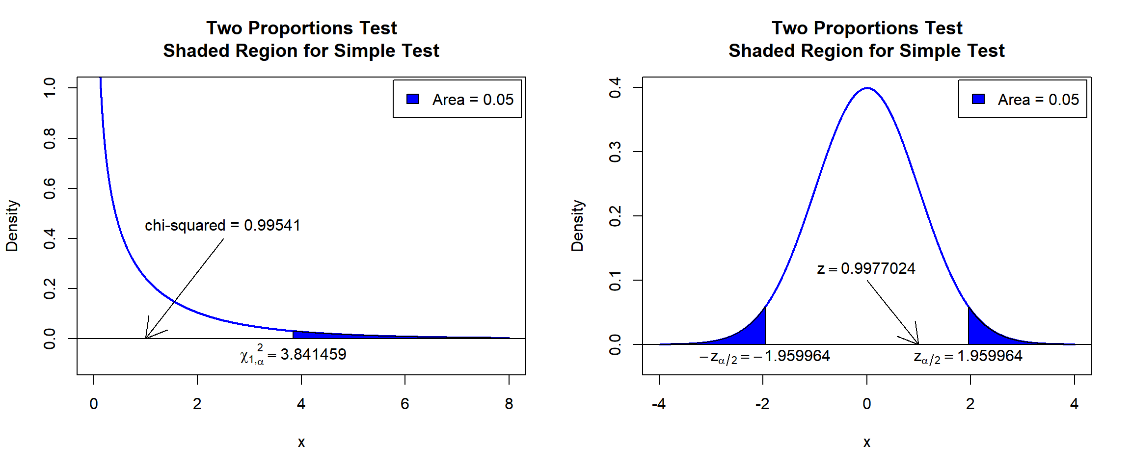
Two Proportions Test Shaded Region for Simple Test in R
See line charts, shading areas under a curve, lines & arrows on plots, mathematical expressions on plots, and legends on plots for more details on making the plot above.
3 Two Proportions Test Critical Value in R
To get the critical value for a two proportions test in R, you can
use the qchisq() function for chi-squared distribution, or
the qnorm() function for the standard normal distribution
to derive the quantile associated with the given level of significance
value \(\alpha\).
For two-tailed test with level of significance \(\alpha\). The critical values are: for chi-squared, qchisq(\(1-\alpha\), 1), or for \(z\), qnorm(\(\alpha/2\)) and qnorm(\(1-\alpha/2\)).
For one-tailed test with level of significance \(\alpha\). The critical value is: for chi-squared, qchisq(\(1-2\alpha\), 1); or for \(z\), left-tailed, qnorm(\(\alpha\)), and for right-tailed, qnorm(\(1-\alpha\)).
Example:
For \(\alpha = 0.1\).
Two-tailed:
[1] 2.705543[1] -1.644854[1] 1.644854One-tailed:
[1] 1.642374[1] -1.281552[1] 1.2815524 Two-tailed Two Proportions Test in R
With number of successes, \(x_1 = 74\) and \(x_2 = 48\), in \(n_1 = 200\) and \(n_2 = 100\) trials.
For the following null hypothesis \(H_0\), and alternative hypothesis \(H_1\), with the level of significance \(\alpha=0.1\), without continuity correction.
\(H_0:\) the difference in population proportions is equal to 0 (\(p_1 - p_2 = 0\)).
\(H_1:\) the difference in population proportions is not equal to 0 (\(p_1 - p_2 \neq 0\), hence the default two-sided).
Because the level of significance is \(\alpha=0.1\), the level of confidence is \(1 - \alpha = 0.9\).
    2-sample test for equality of proportions without continuity correction

data:  c(74, 48) out of c(200, 100)
X-squared = 3.3432, df = 1, p-value = 0.06749
alternative hypothesis: two.sided
90 percent confidence interval:
 -0.20953064 -0.01046936
sample estimates:
prop 1 prop 2
  0.37   0.48
Interpretation:
P-value: With the p-value (\(p = 0.06749\)) being less than the level of significance 0.1, we reject the null hypothesis that the difference in proportions is equal to 0.
\(\chi^2_1\) T-statistic: With test statistics value (\(\chi^2_1 = 3.3432\)) being in the critical region (shaded area), that is, \(\chi^2_1 = 3.3432\) greater than \(\chi^2_{1, \alpha}=\text{qchisq(0.9, 1)}=2.7055435\), we reject the null hypothesis that the difference in proportions is equal to 0.
\(z\) T-statistic: With test statistics value (\(z=-1.828442=\sqrt{\chi^2_1 = 3.3432}\)) being in the critical region (shaded area), that is, \(z=-1.828442\) less than \(-z_{\alpha/2}=\text{qnorm(0.05)}=-1.6448536\) \(=-\sqrt{\text{qchisq(0.9, 1)}=2.7055435}\), we reject the null hypothesis that the difference in proportions is equal to 0.
Confidence Interval: With the null hypothesis difference in proportions value (\(p_1 - p_2 = 0\)) being outside the confidence interval, \([-0.20953064, -0.01046936]\), we reject the null hypothesis that the difference in proportions is equal to 0.
par(mfrow=c(1,2))
#Plot Chi-squared
x = seq(0.01, 8, 1/1000); y = dchisq(x, df=1)
plot(x, y, type = "l",
     xlim = c(0, 8), ylim = c(-0.1, min(max(y), 1)),
     main = "Two Proportions Test
Shaded Region for Two-tailed Test",
     xlab = "x", ylab = "Density",
     lwd = 2, col = "blue")
abline(h=0)
# Add shaded region and legend
point = qchisq(0.9, 1)
polygon(x = c(x[x >= point], 8, point),
        y = c(y[x >= point], 0, 0),
        col = "blue")
legend("topright", c("Area = 0.1"),
       fill = c("blue"), inset = 0.01)
# Add critical value and chi-value
arrows(3.3432, 0.4, 3.3432, 0)
text(3.3432, 0.45, "chi-squared = 3.3432")
text(2.705543, -0.06, expression(chi[1][','][alpha]^2==2.705543))
#Plot z
x = seq(-4, 4, 1/1000); y = dnorm(x)
plot(x, y, type = "l",
     xlim = c(-4, 4), ylim = c(-0.03, max(y)),
     main = "Two Proportions Test
Shaded Region for Two-tailed Test",
     xlab = "x", ylab = "Density",
     lwd = 2, col = "blue")
abline(h=0)
# Add shaded region and legend
point1 = qnorm(0.05); point2 = qnorm(0.95)
polygon(x = c(-4, x[x <= point1], point1),
        y = c(0, y[x <= point1], 0),
        col = "blue")
polygon(x = c(x[x >= point2], 4, point2),
        y = c(y[x >= point2], 0, 0),
        col = "blue")
legend("topright", c("Area = 0.1"),
       fill = c("blue"), inset = 0.01)
# Add critical value and z-value
arrows(0, 0.1, -1.828442, 0)
text(0, 0.12, expression(z==-1.828442))
text(-1.644854, -0.02, expression(-z[alpha/2]==-1.644854))
text(1.644854, -0.02, expression(z[alpha/2]==1.644854))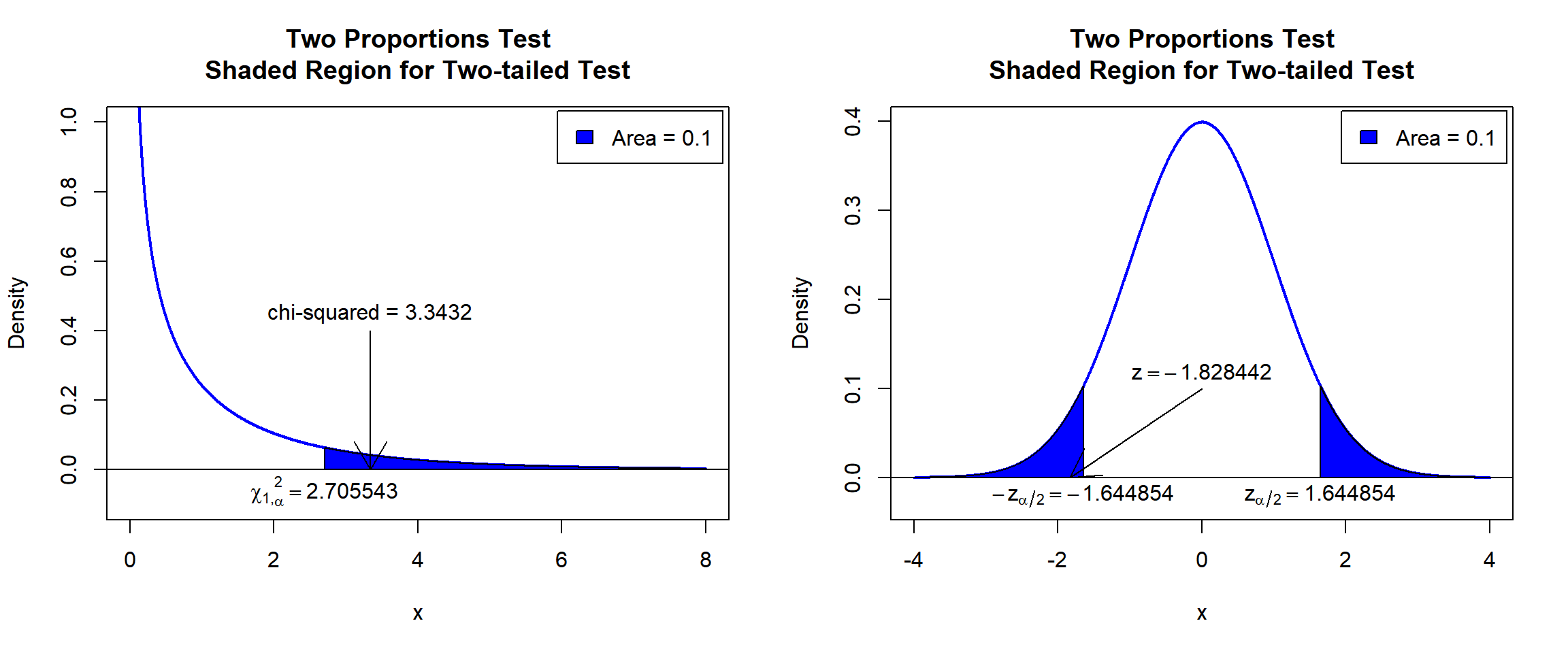
Two Proportions Test Shaded Region for Two-tailed Test in R
5 One-tailed Two Proportions Test in R
Right Tailed Test
With number of successes, \(x_1 = 33\) and \(x_2 = 42\), in \(n_1 = 50\) and \(n_2 = 100\) trials.
For the following null hypothesis \(H_0\), and alternative hypothesis \(H_1\), with the level of significance \(\alpha=0.1\), without continuity correction.
\(H_0:\) the difference in population proportions is equal to 0 (\(p_1 - p_2 = 0\)).
\(H_1:\) proportion 1 is greater than proportion 2 (\(p_1 - p_2 > 0\), hence one-sided).
Because the level of significance is \(\alpha=0.1\), the level of confidence is \(1 - \alpha = 0.9\).
    2-sample test for equality of proportions without continuity correction

data:  c(33, 42) out of c(50, 100)
X-squared = 7.68, df = 1, p-value = 0.002792
alternative hypothesis: greater
90 percent confidence interval:
 0.1333614 1.0000000
sample estimates:
prop 1 prop 2
  0.66   0.42
Interpretation:
P-value: With the p-value (\(p = 0.002792\)) being less than the level of significance 0.1, we reject the null hypothesis that the difference in proportions is equal to 0.
\(\chi^2_1\) T-statistic: With test statistics value (\(\chi^2_1 = 7.68\)) being in the critical region (shaded area), that is, \(\chi^2_1 = 7.68\) greater than \(\chi^2_{1,2\alpha}=\text{qchisq(0.8, 1)}=1.6423744\), we reject the null hypothesis that the difference in proportions is equal to 0.
\(z\) T-statistic: With test statistics value (\(z=2.7712813=\sqrt{\chi^2_1 = 7.68}\)) being in the critical region (shaded area), that is, \(z=2.7712813\) greater than \(z_{\alpha}=\text{qnorm(0.9)}=1.2815516\) \(=\sqrt{\text{qchisq(0.8, 1)}=1.6423744}\), we reject the null hypothesis that the difference in proportions is equal to 0.
Confidence Interval: With the null hypothesis difference in proportions value (\(p_1 - p_2 = 0\)) being outside the confidence interval, \([0.1333614, 1.0)\), we reject the null hypothesis that the difference in proportions is equal to 0.
par(mfrow=c(1,2))
#Plot Chi-squared
x = seq(0.01, 8, 1/1000); y = dchisq(x, df=1)
plot(x, y, type = "l",
     xlim = c(0, 8), ylim = c(-0.1, min(max(y), 1)),
     main = "Two Proportions Test
Shaded Region for Right-tailed Test",
     xlab = "x", ylab = "Density",
     lwd = 2, col = "blue")
abline(h=0)
# Add shaded region and legend
point = qchisq(0.8, 1)
polygon(x = c(x[x >= point], 8, point),
        y = c(y[x >= point], 0, 0),
        col = "blue")
legend("topright", c("Area = 0.2"),
       fill = c("blue"), inset = 0.01)
# Add critical value and chi-value
arrows(5, 0.4, 7.68, 0)
text(5, 0.45, "chi-squared = 7.68")
text(1.642374, -0.06, expression(chi[1][','][2*alpha]^2==1.642374))
#Plot z
x = seq(-4, 4, 1/1000); y = dnorm(x)
plot(x, y, type = "l",
     xlim = c(-4, 4), ylim = c(-0.03, max(y)),
     main = "Two Proportions Test
Shaded Region for Right-tailed Test",
     xlab = "x", ylab = "Density",
     lwd = 2, col = "blue")
abline(h=0)
# Add shaded region and legend
point = qnorm(0.9)
polygon(x = c(x[x >= point], 4, point),
        y = c(y[x >= point], 0, 0),
        col = "blue")
legend("topright", c("Area = 0.1"),
       fill = c("blue"), inset = 0.01)
# Add critical value and z-value
arrows(2.771281, 0.15, 2.771281, 0)
text(2.771281, 0.17, expression(z==2.771281))
text(1.281552, -0.02, expression(z[alpha]==1.281552))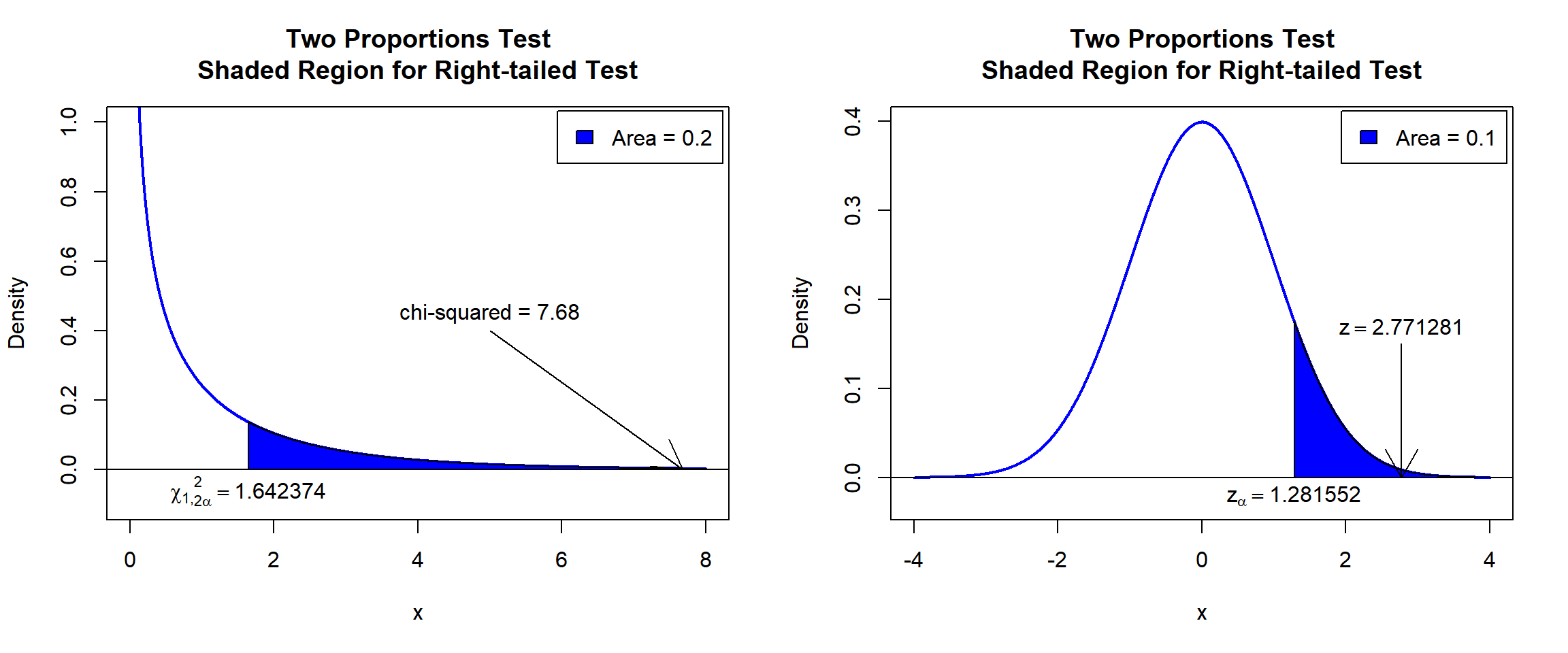
Two Proportions Test Shaded Region for Right-tailed Test in R
Left Tailed Test
With number of successes, \(x_1 = 121\) and \(x_2 = 128\), in \(n_1 = 200\) and \(n_2 = 200\) trials.
For the following null hypothesis \(H_0\), and alternative hypothesis \(H_1\), with the level of significance \(\alpha=0.05\), with continuity correction.
\(H_0:\) the difference in population proportions is equal to 0 (\(p_1 - p_2 = 0\)).
\(H_1:\) proportion 1 is less than proportion 2 (\(p_1 - p_2 < 0\), hence one-sided).
Because the level of significance is \(\alpha=0.05\), the level of confidence is \(1 - \alpha = 0.95\).
    2-sample test for equality of proportions with continuity correction

data:  c(121, 128) out of c(200, 200)
X-squared = 0.38299, df = 1, p-value = 0.268
alternative hypothesis: less
95 percent confidence interval:
 -1.0000000  0.0496842
sample estimates:
prop 1 prop 2
 0.605  0.640
Interpretation:
P-value: With the p-value (\(p = 0.268\)) being greater than the level of significance 0.05, we fail to reject the null hypothesis that the difference in proportions is equal to 0.
\(\chi^2_1\) T-statistic: With test statistics value (\(\chi^2_1 = 0.38299\)) being less than the critical value, \(\chi^2_{1,2\alpha}=\text{qchisq(0.9, 1)}=2.7055435\) (or not in the shaded region), we fail to reject the null hypothesis that the difference in proportions is equal to 0.
\(z\) T-statistic: With test statistics value (\(z=-0.6188619=-\sqrt{\chi^2_1 = 0.38299}\)) being greater than the critical value, \(-z_{\alpha}=\text{qnorm(0.05)}=-1.6448536\) \(=-\sqrt{\text{qchisq(0.9, 1)}=2.7055435}\) (or not in the shaded region), we fail to reject the null hypothesis that the difference in proportions is equal to 0.
Confidence Interval: With the null hypothesis difference in proportions value (\(p_1 - p_2 = 0\)) being inside the confidence interval, \((-1.0, 0.0496842]\), we fail reject the null hypothesis that the difference in proportions is equal to 0.
par(mfrow=c(1,2))
#Plot Chi-squared
x = seq(0.01, 8, 1/1000); y = dchisq(x, df=1)
plot(x, y, type = "l",
     xlim = c(0, 8), ylim = c(-0.1, min(max(y), 1)),
     main = "Two Proportions Test
Shaded Region for Left-tailed Test",
     xlab = "x", ylab = "Density",
     lwd = 2, col = "blue")
abline(h=0)
# Add shaded region and legend
point = qchisq(0.9, 1)
polygon(x = c(x[x >= point], 8, point),
        y = c(y[x >= point], 0, 0),
        col = "blue")
legend("topright", c("Area = 0.1"),
       fill = c("blue"), inset = 0.01)
# Add critical value and chi-value
arrows(2.5, 0.4, 0.38299, 0)
text(2.5, 0.45, "chi-squared = 0.38299")
text(2.705543, -0.06, expression(chi[1][','][2*alpha]^2==2.705543))
#Plot z
x = seq(-4, 4, 1/1000); y = dnorm(x)
plot(x, y, type = "l",
     xlim = c(-4, 4), ylim = c(-0.03, max(y)),
     main = "Two Proportions Test
Shaded Region for Left-tailed Test",
     xlab = "x", ylab = "Density",
     lwd = 2, col = "blue")
abline(h=0)
# Add shaded region and legend
point = qnorm(0.05)
polygon(x = c(-4, x[x <= point], point),
        y = c(0, y[x <= point], 0),
        col = "blue")
legend("topright", c("Area = 0.05"),
       fill = c("blue"), inset = 0.01)
# Add critical value and z-value
arrows(0, 0.15, -0.6188619, 0)
text(0, 0.17, expression(z==-0.6188619))
text(-1.644854, -0.02, expression(-z[alpha]==-1.644854))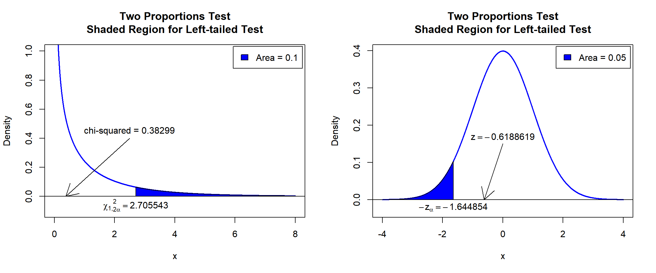
Two Proportions Test Shaded Region for Left-tailed Test in R
6 Two Proportions Test with Known Null Proportions in R
For the cases where the null population proportions are specified, in R, this is equivalent to having two separate one proportion chi-squared tests for \(p_1\) and \(p_2\), then summing the two \(\chi^2_1\) test statistic values (both with 1 degree of freedom) to have a \(\chi^2_2\) test statistics (with 2 degrees of freedom). This test is also only applicable for the two sided alternative.
Sample:
With number of successes, \(x_1 = 54\) and \(x_2 = 35\), in \(n_1 = 100\) and \(n_2 = 80\) trials, and \(p_1 = 0.6\) and \(p_2 = 0.4\).
For the following null hypothesis \(H_0\), and alternative hypothesis \(H_1\), with the level of significance \(\alpha=0.1\), without continuity correction.
\(H_0:\) the difference in population proportions is equal to 0.2 (\(p_1 - p_2 = 0.6 - 0.4\)).
\(H_1:\) the difference in population proportions is not equal to 0.2 (\(p_1 - p_2 \neq 0.6 - 0.4\), hence the applicable two-sided).
    2-sample test for given proportions without continuity correction

data:  c(x1 = 54, x2 = 35) out of c(n1 = 100, n2 = 80), null probabilities c(0.6, 0.4)
X-squared = 1.9688, df = 2, p-value = 0.3737
alternative hypothesis: two.sided
null values:
prop 1 prop 2
   0.6    0.4
sample estimates:
prop 1 prop 2
0.5400 0.4375
P-values and \(\chi^2\) test statistics should be interpreted similarly to the examples above.
7 Two Proportions Test: Test Statistics, P-value & Degree of Freedom in R
Here for a two proportions test, we show how to get the test
statistics (or chi-squared value), p-values, and degrees of freedom from
the prop.test() function in R, or by written code.
x = c(47, 53); n = c(100, 100)
prop_object = prop.test(x, n,
                      alternative = "two.sided",
                      conf.level = 0.95,
                      correct = TRUE)
prop_object
    2-sample test for equality of proportions with continuity correction

data:  x out of n
X-squared = 0.5, df = 1, p-value = 0.4795
alternative hypothesis: two.sided
95 percent confidence interval:
 -0.20834069  0.08834069
sample estimates:
prop 1 prop 2
  0.47   0.53
To get the test statistic or chi-squared value:
\[z = \frac{(\frac{x_1}{n_1}-\frac{x_2}{n_2})}{\sqrt {\hat p(1-\hat p) \left(\frac{1}{n_1} + \frac{1}{n_2} \right)}} \quad \text{or} \quad \chi^2_1=\sum_{i,j=1}^{2}\frac{(O_{ij}-E_{ij})^2}{E_{ij}},\]
where
\[\hat p = \frac{x_1 + x_2}{n_1 + n_2}.\]
Applying Yates’ continuity correction, it takes the form:
\[z = \frac{(\frac{x_1 \pm c}{n_1}-\frac{x_2 \pm c}{n_2})}{\sqrt {\hat p(1-\hat p) \left(\frac{1}{n_1} + \frac{1}{n_2} \right)}} \quad \text{or} \quad \chi^2_1=\sum_{i,j=1}^{2}\frac{(|O_{ij}-E_{ij}|-c)^2}{E_{ij}}.\]
\(c = \min\{0.5, k\}\), with \(k = |n_2x_1-n_1x_2|/(n_1+n_2)\)
For
\(i = \{1, 2\}\), \(x_i+c \;\) when \(n_i \hat p \geq x_i\), and \(x_i-c \;\) when \(n_i \hat p < x_i\).
X-squared
0.5 [1] 0.5Same as (with continuity correction):
x1 = 47; x2 = 53; n1 = 100; n2 = 100; phat = (x1+x2)/(n1+n2)
k = abs(n2*x1-n1*x2)/(n1+n2); c = min(0.5, k)
#z
cc1 = c*sign(n1*phat-x1) # n1*phat > x1, so we use x1+c correction
cc2 = c*sign(n2*phat-x2) # n2*phat < x2, so we use x2-c correction
z = ((x1+cc1)/n1 - (x2+cc2)/n2)/sqrt(phat*(1-phat)*(1/n1+1/n2))
z
[1] -0.7071068[1] 0.5#chi-squared
obs = c(x1, x2, n1-x1, n2-x2)
exp = c(n1*phat, n2*phat, n1*(1-phat), n2*(1-phat))
chi = sum(((abs(obs-exp)-c)^2)/exp)
chi[1] 0.5Without continuity correction:
x1 = 47; x2 = 53; n1 = 100; n2 = 100; phat = (x1+x2)/(n1+n2)
#z
z = (x1/n1 - x2/n2)/sqrt(phat*(1-phat)*(1/n1+1/n2))
z
z^2 # convert to chi-squared
#chi-squared
obs = c(x1, x2, n1-x1, n2-x2)
exp = c(n1*phat, n2*phat, n1*(1-phat), n2*(1-phat))
chi = sum((abs(obs-exp)^2)/exp)
chi
To get the p-value:
Two-tailed: With \(z = \sqrt{\chi^2_1}\): for positive test statistic (\(z^+\)), and negative test statistic (\(z^-\)).
For \(\chi^2_1\), \(P \left(\chi^2_1> \text{observed} \right)\)
For \(z\), \(Pvalue = 2*P(Z>z^+)\) or \(Pvalue = 2*P(Z<z^-)\).
One-tailed: For \(\chi^2_1\) is \(\frac{1}{2}*P \left(\chi^2_1> \text{observed} \right)\)
For \(z\), for right-tail, \(Pvalue = P(Z>z^+)\) or for left-tail, \(Pvalue = P(Z<z^-)\).
[1] 0.4795001Same as:
Note that the p-value depends on the \(\text{test statistics}\) (\(\chi^2_1 = 0.5\)), \(\text{degrees of freedom}\) (1), and \(z = -\sqrt{\chi^2_1} = -0.7071068\). We
also use the distribution functions pchisq() for the
chi-squared distribution and pnorm() for the standard
normal distribution in R.
[1] 0.4795001[1] 0.4795001[1] 0.4795001To get the degrees of freedom:
The degree of freedom is \(1\).
df
1 [1] 18 Two Proportions Test: Estimates & Confidence Interval in R
Here for a two proportions test, we show how to get the sample
proportions and confidence interval from the prop.test()
function in R, or by written code.
x = c(x1 = 26, x2 = 23); n = c(n1 = 50, n2 = 50)
prop_object = prop.test(x, n,
                      alternative = "two.sided",
                      conf.level = 0.9,
                      correct = TRUE)
prop_object
    2-sample test for equality of proportions with continuity correction

data:  x out of n
X-squared = 0.16006, df = 1, p-value = 0.6891
alternative hypothesis: two.sided
90 percent confidence interval:
 -0.1241561  0.2441561
sample estimates:
prop 1 prop 2
  0.52   0.46
To get the point estimates or sample proportions:
\[\hat p_1 = \frac{x_1}{n_1}, \quad \hat p_2 = \frac{x_2}{n_2}.\]
prop 1 prop 2
0.52 0.46 [1] 0.52 0.46Same as:
[1] 0.52[1] 0.46To get the confidence interval for \(p_1 - p_2\) with continuity correction:
Set \(c = \min\{0.5, k\}\), with \(k = |n_2x_1-n_1x_2|/(n_1+n_2)\).
With \(\hat p_1 = \frac{x_1}{n_1}\), \(\hat p_2 = \frac{x_2}{n_2}\), and un-pooled standard error estimate, \(\widehat {SE} = \sqrt {\frac{\hat p_1(1-\hat p_1)}{n_1} + \frac{\hat p_2(1-\hat p_2)}{n_2}}\).
For two-tailed:
The lower bound is:
\[\left\{\hat p_1 - \hat p_2 - \frac{(n_1+n_2)c}{n_1n_2}\right\} - z_{\alpha/2}* \widehat {SE}.\] The upper bound is:
\[\left\{\hat p_1 - \hat p_2 + \frac{(n_1+n_2)c}{n_1n_2}\right\} + z_{\alpha/2}* \widehat {SE}.\]
For right one-tailed:
\[CI = \left[\left\{\hat p_1 - \hat p_2 - \frac{(n_1+n_2)c}{n_1n_2}\right\} - z_{\alpha}* \widehat {SE} \;,\; 1 \right].\]
For left one-tailed:
\[CI = \left[-1 \;,\; \left\{\hat p_1 - \hat p_2 + \frac{(n_1+n_2)c}{n_1n_2}\right\} + z_{\alpha}* \widehat {SE} \right].\]
[1] -0.1241561  0.2441561
attr(,"conf.level")
[1] 0.9[1] -0.1241561 0.2441561Same as:
x1 = 26; x2 = 23; n1 = 50; n2 = 50; alpha = 0.1
# Set c = 0 for no continuity correction
k = abs(n2*x1-n1*x2)/(n1+n2); c = min(0.5, k)
ph1 = x1/n1; ph2 = x2/n2
SE = sqrt(ph1*(1-ph1)/n1 + ph2*(1-ph2)/n2)
l = (ph1 - ph2 - (n1+n2)*c/(n1*n2)) - qnorm(1-alpha/2)*SE
u = (ph1 - ph2 + (n1+n2)*c/(n1*n2)) + qnorm(1-alpha/2)*SE
c(l, u)
[1] -0.1241561 0.2441561One tailed example:
x1 = 26; x2 = 23; n1 = 50; n2 = 50; alpha = 0.1
# Set c = 0 for no continuity correction
k = abs(n2*x1-n1*x2)/(n1+n2); c = min(0.5, k)
ph1 = x1/n1; ph2 = x2/n2
SE = sqrt(ph1*(1-ph1)/n1 + ph2*(1-ph2)/n2)
# Right Tail
l = (ph1 - ph2 - (n1+n2)*c/(n1*n2)) - qnorm(1-alpha)*SE
c(l, 1)
# Left Tail
u = (ph1 - ph2 + (n1+n2)*c/(n1*n2)) + qnorm(1-alpha)*SE
c(-1, u)
To get the confidence interval for \(p_1 - p_2\) without continuity correction:
With \(\hat p_1 = \frac{x_1}{n_1}\), \(\hat p_2 = \frac{x_2}{n_2}\), and un-pooled standard error estimate, \(\widehat {SE} = \sqrt {\frac{\hat p_1(1-\hat p_1)}{n_1} + \frac{\hat p_2(1-\hat p_2)}{n_2}}\).
For two-tailed:
\[\left[ \left\{\hat p_1 - \hat p_2 \right\} - z_{\alpha/2}* \widehat {SE} \;,\; \left\{\hat p_1 - \hat p_2 \right\} + z_{\alpha/2}* \widehat {SE} \right].\]
For right one-tailed:
\[CI = \left[\left\{\hat p_1 - \hat p_2\right\} - z_{\alpha}* \widehat {SE} \;,\; 1 \right].\]
For left one-tailed:
\[CI = \left[-1 \;,\; \left\{\hat p_1 - \hat p_2\right\} + z_{\alpha}* \widehat {SE} \right].\]
Same as:
x1 = 26; x2 = 23; n1 = 50; n2 = 50; alpha = 0.1
ph1 = x1/n1; ph2 = x2/n2
SE = sqrt(ph1*(1-ph1)/n1 + ph2*(1-ph2)/n2)
l = (ph1 - ph2) - qnorm(1-alpha/2)*SE
u = (ph1 - ph2) + qnorm(1-alpha/2)*SE
c(l, u)
One tailed example:
The feedback form is a Google form but it does not collect any personal information.
Please click on the link below to go to the Google form.
Thank You!
Go to Feedback Form
Copyright © 2020 - 2026. All Rights Reserved by Stats Codes