1 Table of Gamma Distribution Functions in R
2 Plot of Gamma Distributions in R
3 Examples for Setting Parameters for Gamma Distributions in R
4 rgamma(): Random Sampling from Gamma Distributions in R
5 dgamma(): Probability Density Function for Gamma Distributions in R
6 pgamma(): Cumulative Distribution Function for Gamma Distributions in R
7 qgamma(): Derive Quantile for Gamma Distributions in R

Here, we discuss gamma distribution functions in R, plots, parameter setting, random sampling, density, cumulative distribution and quantiles.

The gamma distribution with parameters \(\tt{shape}=\alpha\), and \(\tt{rate}=\lambda\) (or \(\tt{scale}=\theta=1/\lambda\)) has probability density function (pdf) formula as:

\[\begin{align} f(x) & = \frac{\lambda^\alpha}{\Gamma(\alpha)} x^{\alpha - 1} e^{-\lambda x } \\ & = \frac{1}{\Gamma(\alpha) \theta^\alpha} x^{\alpha - 1} e^{-\frac{x}{\theta}},\end{align}\]

for \(x \geq 0\), where \(\alpha > 0\), \(\lambda > 0\) (or \(\theta > 0\)),

and \(\Gamma\) is the \(\tt{gamma\;function}\).

The mean is \(\frac{\alpha}{\lambda}\) (or \(\alpha\theta\)), and the variance is \(\frac{\alpha}{\lambda^2}\) (or \(\alpha\theta^2\)).

1 Table of Gamma Distribution Functions in R

The table below shows the functions for gamma distributions in R.

Table of Gamma Distribution Functions in R
Function	Usage
rgamma(n, shape, rate=1, scale=1/rate)	Simulate a random sample with \(n\) observations
dgamma(x, shape, rate=1, scale=1/rate)	Calculate the probability density at the point \(x\)
pgamma(q, shape, rate=1, scale=1/rate)	Calculate the cumulative distribution at the point \(q\)
qgamma(p, shape, rate=1, scale=1/rate)	Calculate the quantile value associated with \(p\)

The examples here are based on the \(\tt{shape}\) and \(\tt{rate}\) parameters in the pdf above, as only one of the "rate" and "scale" arguments can be specified at a time. Hence, the "scale" argument (for \(\tt{scale}\)) is excluded in the examples below.

However, to use the \(\tt{scale}\) parameter, you can set the argument to the scale value of the distribution. For example:

dgamma(2.5, shape = 1.5, scale = 3)

[1] 0.1492214

Which (since \(\tt{rate = 1/scale}\)) is equivalent to:

dgamma(2.5, shape = 1.5, rate = 1/3)

[1] 0.1492214

2 Plot of Gamma Distributions in R

Single distribution:

Below is a plot of the gamma distribution function with \(\tt{shape}=3\) and \(\tt{rate}=1/2\).

x = seq(0, 24, 1/1000); y = dgamma(x, 3, 1/2)
plot(x, y, type = "l",
     xlim = c(0, 24), ylim = c(0, max(y)),
     main = "Probability Density Function of Gamma Distribution (3, 1/2)",
     xlab = "x", ylab = "Density",
     lwd = 2, col = "blue")
# Add legend
legend("topright", "Shape = 3 Rate = 1/2",
       lwd = 2,
       col = "blue",
       bty = "n")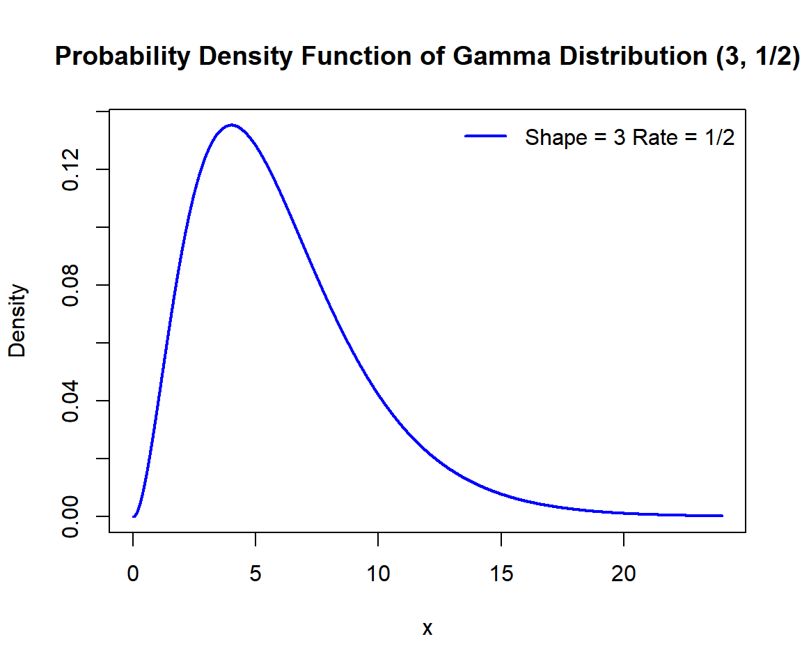

Probability Density Function (PDF) of a Gamma Distribution in R

Multiple distributions:

Below is a plot of the multiple gamma distribution functions in one graph.

x1 = seq(0, 25, 1/1000); y1 = dgamma(x1, 2, 1/3)
x2 = seq(0, 25, 1/1000); y2 = dgamma(x2, 2, 1/2)
x3 = seq(0, 25, 1/1000); y3 = dgamma(x3, 4, 1/2)
plot(x1, y1, type = "l",
     xlim = c(0, 25), ylim = range(c(y1, y2, y3)),
     main = "Probability Density Functions of Gamma Distributions",
     xlab = "x", ylab = "Density",
     lwd = 2, col = "blue")
points(x2, y2, type = "l", lwd = 2, col = "red")
points(x3, y3, type = "l", lwd = 2, col = "green")
# Add legend
legend("topright", c("shape = 2, rate = 1/3",
                    "shape = 2, rate = 1/2",
                    "shape = 4, rate = 1/2"),
       lwd = c(2, 2, 2),
       col = c("blue", "red", "green"),
       bty = "n")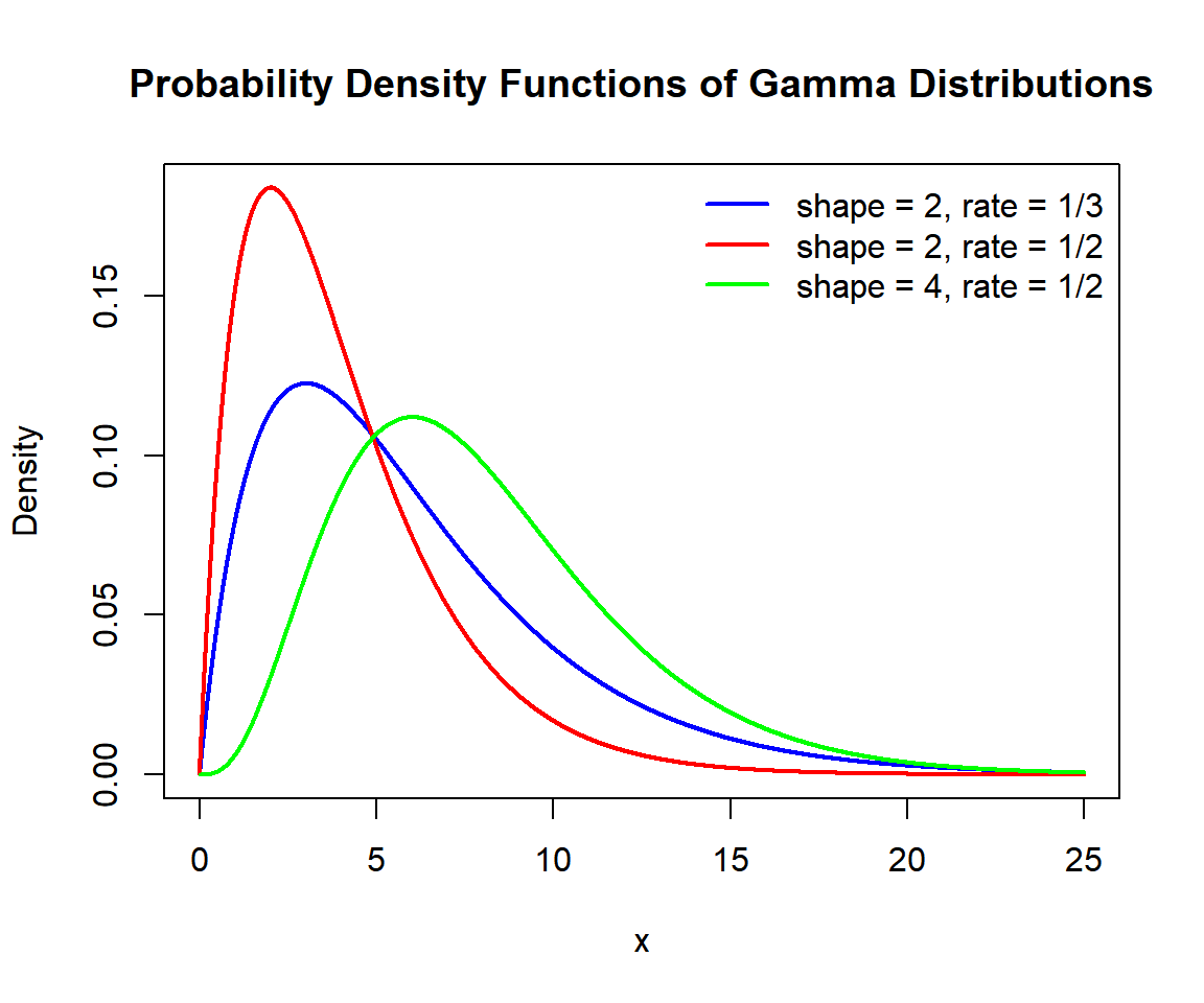

Probability Density Functions (PDFs) of Gamma Distributions in R

3 Examples for Setting Parameters for Gamma Distributions in R

To set the parameters for the gamma distribution function, with \(\tt{shape}=4.5\) and \(\tt{rate}=1/3\).

For example, for dgamma(), the following are the same:

# The order of 4.5 and 1/3 matters here as the parameter names are not used.
# The first number 4.5 is shape, and 1/3 is rate.
dgamma(5.5, 4.5, 1/3)

[1] 0.03822724

# Or:
dgamma(5.5, shape = 4.5, rate = 1/3)

[1] 0.03822724

# Or:
dgamma(5.5, rate = 1/3, shape = 4.5)

[1] 0.03822724

4 rgamma(): Random Sampling from Gamma Distributions in R

Sample 1200 observations from the gamma distribution with \(\tt{shape}=6\) and \(\tt{rate}=1/2.5\):

rgamma(1200, 6, 1/2.5)

set.seed(123) # Line allows replication (use any number).
sample = rgamma(1200, 6, 1/2.5)
hist(sample,
     main = "Histogram of 1200 Observations from Gamma Distribution
with Shape = 6 and Rate = 1/2.5",
     xlab = "x",
     col = "deepskyblue", border = "white")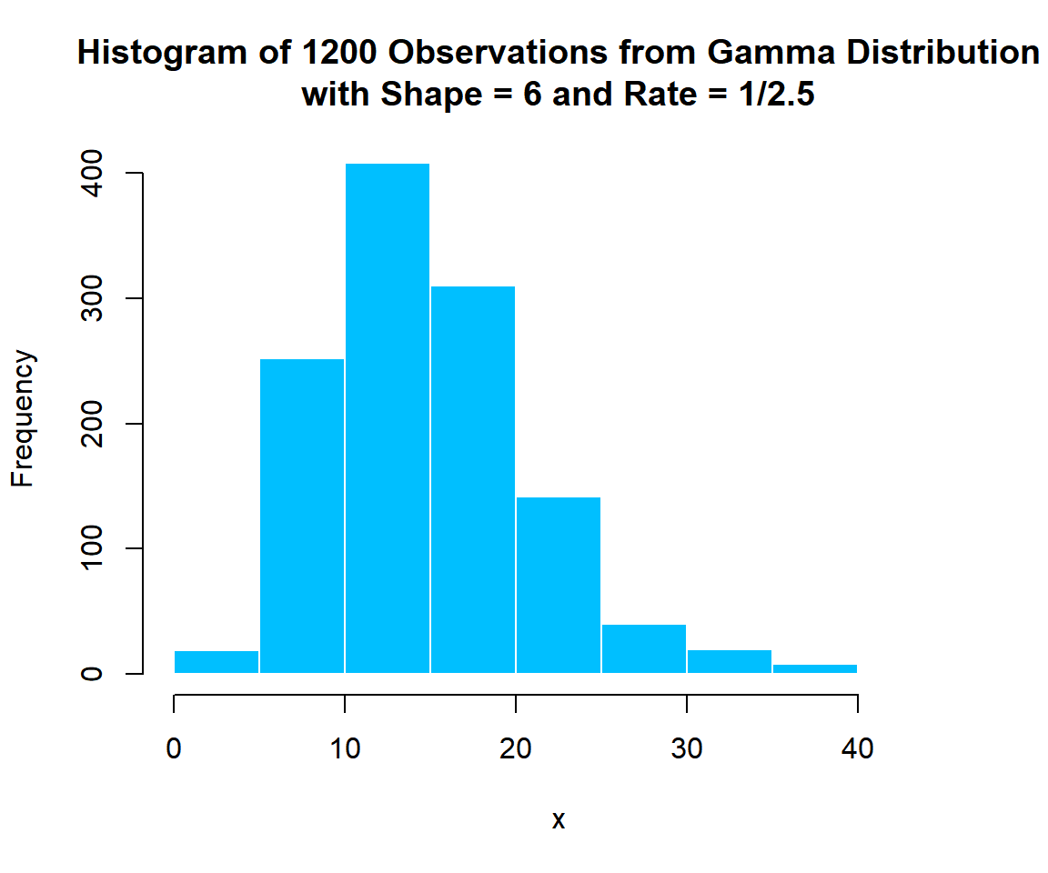

Histogram of Gamma Distribution (6, 1/2.5) Random Sample in R

5 dgamma(): Probability Density Function for Gamma Distributions in R

Calculate the density at \(x = 4.6\), in the gamma distribution with \(\tt{shape}=5.5\) and \(\tt{rate}=0.6\):

dgamma(4.6, 5.5, 0.6)

[1] 0.06994112

x = seq(0, 25, 1/1000); y = dgamma(x, 5.5, 0.6)
plot(x, y, type = "l",
     xlim = c(0, 25), ylim = c(0, max(y)),
     main = "Probability Density Function of Gamma Distribution
with Shape = 5.5 and Rate = 0.6",
     xlab = "x", ylab = "Density",
     lwd = 2, col = "blue")
# Add lines
segments(4.6, -1, 4.6, 0.06994112)
segments(-1, 0.06994112, 4.6, 0.06994112)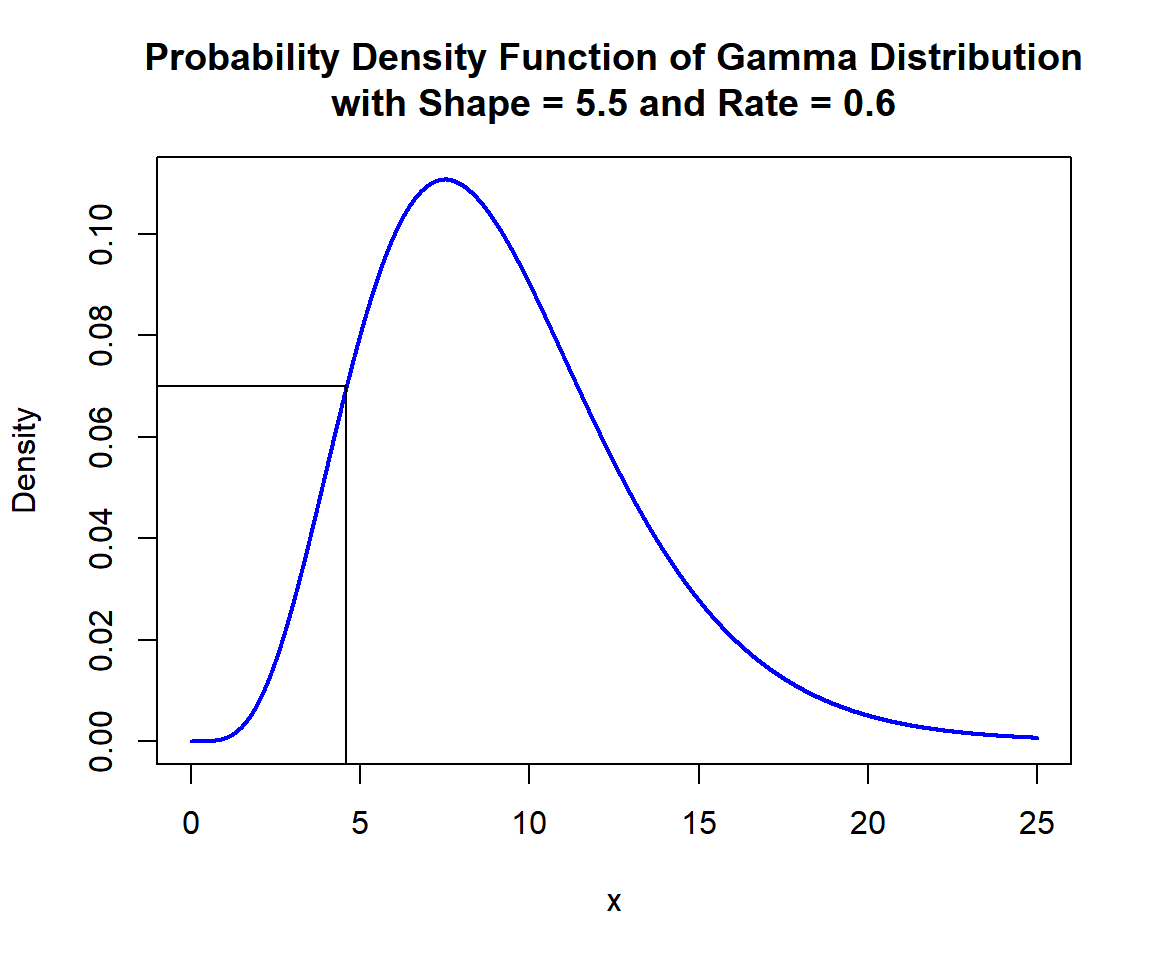

Probability Density Function (PDF) of Gamma Distribution (5.5, 0.6) in R

6 pgamma(): Cumulative Distribution Function for Gamma Distributions in R

Calculate the cumulative distribution at \(x = 8.5\), in the gamma distribution with \(\tt{shape}=4\) and \(\tt{rate}=1/2\). That is, \(P(X \le 8.5)\):

pgamma(8.5, 4, 1/2)

[1] 0.6137884

x = seq(0, 25, 1/1000); y = pgamma(x, 4, 1/2)
plot(x, y, type = "l",
     xlim = c(0, 25), ylim = c(0,1),
     main = "Cumulative Distribution Function of Gamma Distribution
Shape = 4 and Rate = 1/2",
     xlab = "x", ylab = "Cumulative Distribution",
     lwd = 2, col = "blue")
# Add lines
segments(8.5, -1, 8.5, 0.6137884)
segments(-1, 0.6137884, 8.5, 0.6137884)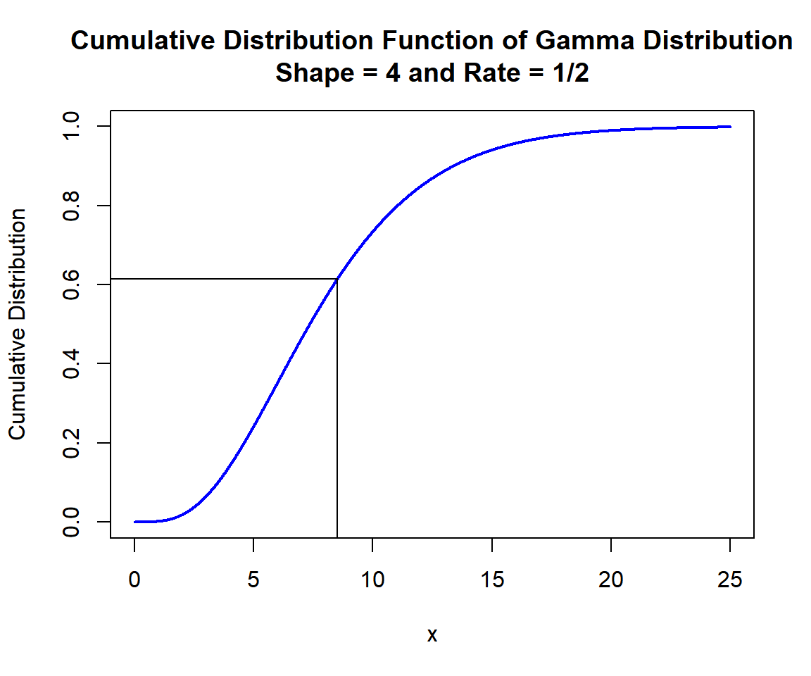

Cumulative Distribution Function (CDF) of Gamma Distribution (4, 1/2) in R

x = seq(0, 25, 1/1000); y = dgamma(x, 4, 1/2)
plot(x, y, type = "l",
     xlim = c(0, 25), ylim = c(0, max(y)),
     main = "Probability Density Function of Gamma Distribution
Shape = 4 and Rate = 1/2",
     xlab = "x", ylab = "Density",
     lwd = 2, col = "blue")
# Add shaded region and legend
point = 8.5
polygon(x = c(x[x <= point], point),
        y = c(y[x <= point], 0),
        col = "limegreen")
legend("topright", c("Area = 0.6137884"),
       fill = c("limegreen"),
       inset = 0.01)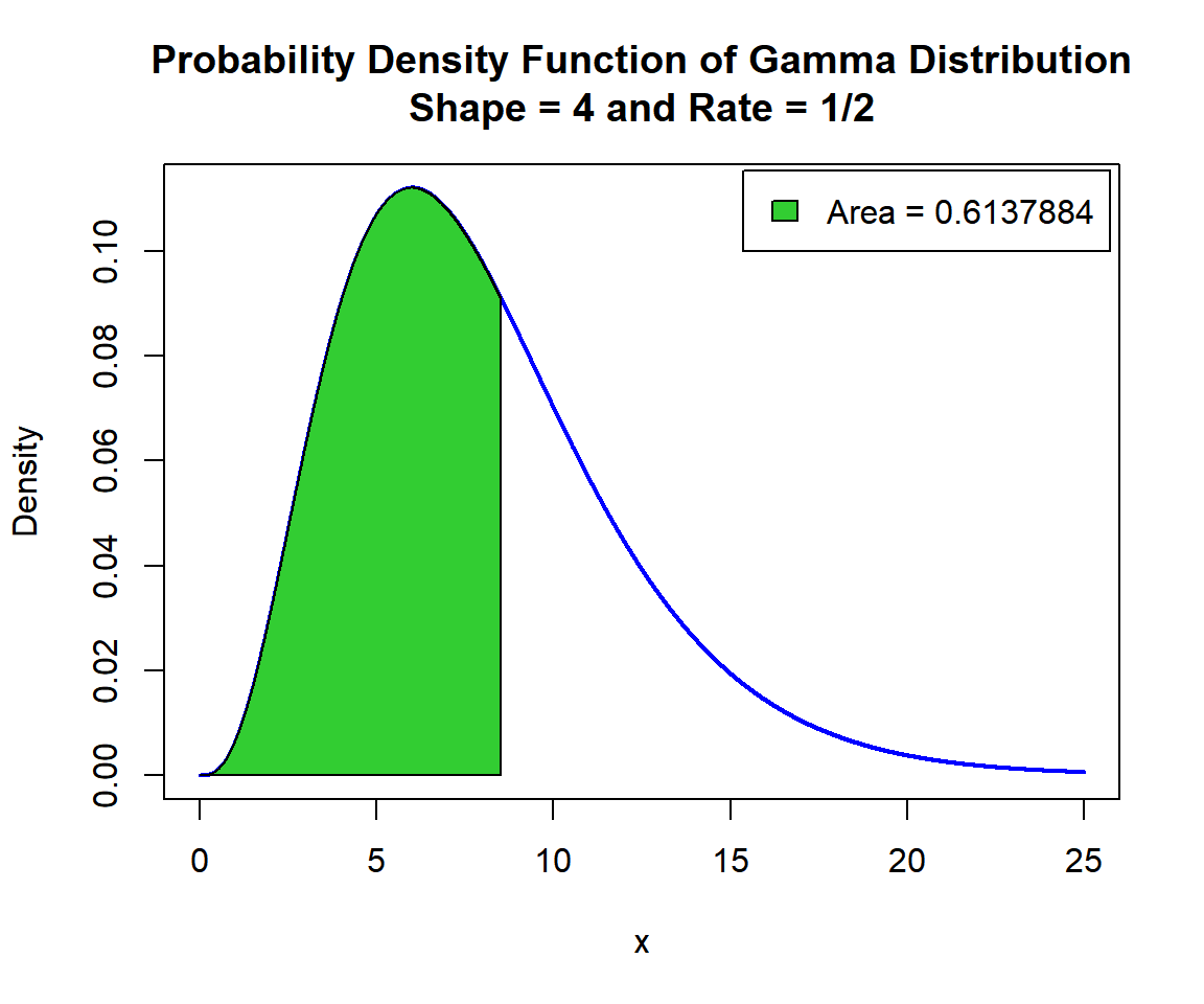

Shaded Probability Density Function (PDF) of Gamma Distribution (4, 1/2) in R

For upper tail, at \(x = 8.5\), that is, \(P(X \ge 8.5) = 1 - P(X \le 8.5)\), set the "lower.tail" argument:

pgamma(8.5, 4, 1/2, lower.tail = FALSE)

[1] 0.3862116

x = seq(0, 25, 1/1000); y = dgamma(x, 4, 1/2)
plot(x, y, type = "l",
     xlim = c(0, 25), ylim = c(0, max(y)),
     main = "Shaded Upper Region: Probability Density Function of
Gamma Distribution with Shape = 4 and Rate = 1/2",
     xlab = "x", ylab = "Density",
     lwd = 2, col = "blue")
# Add shaded region and legend
point = 8.5
polygon(x = c(point, x[x >= point]),
        y = c(0, y[x >= point]),
        col = "limegreen")
legend("topright", c("Area = 0.3862116"),
       fill = c("limegreen"),
       inset = 0.01)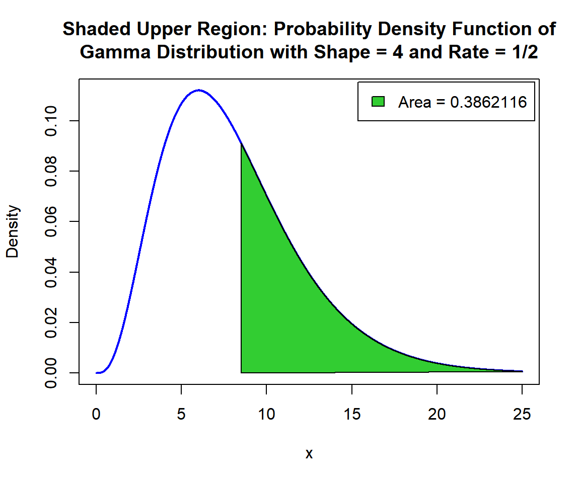

Shaded Upper Region: Probability Density Function (PDF) of Gamma Distribution (4, 1/2) in R

7 qgamma(): Derive Quantile for Gamma Distributions in R

Derive the quantile for \(p = 0.95\), in the gamma distribution with \(\tt{shape}=6.5\) and \(\tt{rate}=0.3\). That is, \(x\) such that, \(P(X \le x)=0.95\):

qgamma(0.95, 6.5, 0.3)

[1] 37.27005

x = seq(0, 60, 1/1000); y = pgamma(x, 6.5, 0.3)
plot(x, y, type = "l",
     xlim = c(0, 60), ylim = c(0,1),
     main = "Cumulative Distribution Function of Gamma Distribution
with Shape = 6.5 and Rate = 0.3",
     xlab = "x", ylab = "Cumulative Distribution",
     lwd = 2, col = "blue")
# Add lines
segments(37.27005, -1, 37.27005, 0.95)
segments(-3, 0.95, 37.27005, 0.95)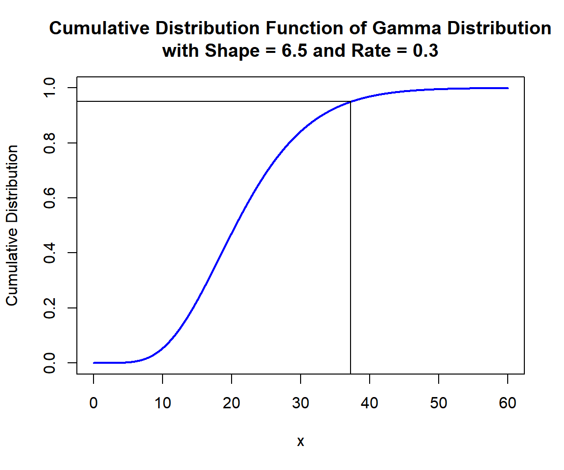

Cumulative Distribution Function (CDF) of Gamma Distribution (6.5, 0.3) in R

x = seq(0, 60, 1/1000); y = dgamma(x, 6.5, 0.3)
plot(x, y, type = "l",
     xlim = c(0, 60), ylim = c(0, max(y)),
     main = "Probability Density Function of Gamma Distribution
with Shape = 6.5 and Rate = 0.3",
     xlab = "x", ylab = "Density",
     lwd = 2, col = "blue")
# Add shaded region and legend
point = 37.27005
polygon(x = c(x[x <= point], point),
        y = c(y[x <= point], 0),
        col = "limegreen")
legend("topright", c("Area = 0.95"),
       fill = c("limegreen"),
       inset = 0.01)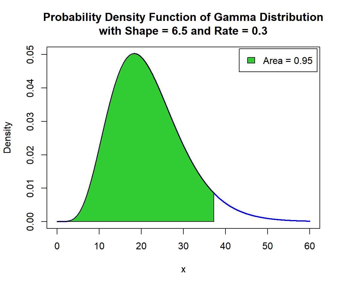

Shaded Probability Density Function (PDF) of Gamma Distribution (6.5, 0.3) in R

For upper tail, for \(p = 0.05\), that is, \(x\) such that, \(P(X \ge x)=0.05\):

qgamma(0.05, 6.5, 0.3, lower.tail = FALSE)

[1] 37.27005

x = seq(0, 60, 1/1000); y = dgamma(x, 6.5, 0.3)
plot(x, y, type = "l",
     xlim = c(0, 60), ylim = c(0, max(y)),
     main = "Shaded Upper Region: Probability Density Function of
Gamma Distribution with Shape = 6.5 and Rate = 0.3",
     xlab = "x", ylab = "Density",
     lwd = 2, col = "blue")
# Add shaded region and legend
point = 37.27005
polygon(x = c(point, x[x >= point]),
        y = c(0, y[x >= point]),
        col = "limegreen")
legend("topright", c("Area = 0.05"),
       fill = c("limegreen"),
       inset = 0.01)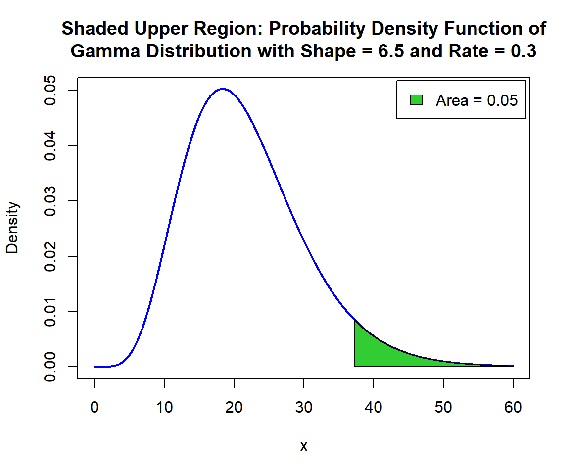

Shaded Upper Region: Probability Density Function (PDF) of Gamma Distribution (6.5, 0.3) in R