Binomial Family Genaralized Linear Model (GLM) in R
Here, we discuss the binomial family GLM in R with interpretations, and link functions including, logit, probit, cauchit, log, and cloglog.
The binomial family generalized linear model in
R can be performed with the glm() function from the base
"stats" package.
The binomial family GLM can be used to study the relationship, if they exist, between a Bernoulli or binomial distributed dependent variable \((y)\), and a set of independent variables \((X = x_1, x_2, \ldots, x_m)\).
The binomial family GLM framework is based on the theoretical assumption that:
\[y\sim Bernoulli(p),\]
with \(p = E(y|X) = E(y|x_1, x_2, \ldots, x_m)\),
\[\begin{align} g(p) & = g(E(y|X)) \\ & = \beta_0 + \beta_1 x_1 + \beta_2 x_2 + \cdots + \beta_m x_m. \end{align}\]
The binomial family GLM then estimates the true coefficients, \(\beta_1, \beta_2, \ldots, \beta_m\), as
\(\widehat \beta_1, \widehat \beta_2, \ldots,
\widehat \beta_m\), and the true intercept, \(\beta_0\), as \(\widehat \beta_0\).
Then for any \(x_1, x_2, \ldots, x_m\) values, these are
used to predict or estimate the true \(p\), as \(\widehat p\), with the equation below:
\[\widehat p = g^{-1}\left( \widehat \beta_0 + \widehat \beta_1 x_1 + \widehat \beta_2 x_2 + \cdots + \widehat \beta_m x_m \right).\]
See also logistic regression.
Sample Steps to Run a Binomial Family Generalized Linear Model:
# Create the data samples for the binomial family GLM
# Values are matched based on matching position in each sample

y = c(1, 1, 0, 0, 1, 0, 0, 0, 1, 1, 0, 1)
x1 = c(4.19, 5.59, 3.50, 2.95, 4.93, 5.60,
       4.57, 4.94, 5.43, 5.14, 3.97, 5.30)
x2 = c(2.15, 2.67, 2.52, 2.79, 2.30, 2.97,
       3.13, 3.34, 2.26, 3.14, 2.89, 2.52)
bf_data = data.frame(y, x1, x2)
bf_data

# Run the binomial family GLM

model = glm(y ~ x1 + x2, family = binomial(link = "logit"))
summary(model)

#or

model = glm(y ~ x1 + x2, family = binomial(link = "logit"),
            data = bf_data)
summary(model)
y x1 x2
1 1 4.19 2.15
2 1 5.59 2.67
3 0 3.50 2.52
4 0 2.95 2.79
5 1 4.93 2.30
6 0 5.60 2.97
7 0 4.57 3.13
8 0 4.94 3.34
9 1 5.43 2.26
10 1 5.14 3.14
11 0 3.97 2.89
12 1 5.30 2.52
Call:
glm(formula = y ~ x1 + x2, family = binomial(link = "logit"))

Coefficients:
            Estimate Std. Error z value Pr(>|z|)
(Intercept)    4.026      8.866   0.454   0.6498
x1             2.479      1.497   1.656   0.0977 .
x2            -5.725      3.192  -1.793   0.0729 .
---
Signif. codes:  0 '***' 0.001 '**' 0.01 '*' 0.05 '.' 0.1 ' ' 1

(Dispersion parameter for binomial family taken to be 1)

    Null deviance: 16.6355  on 11  degrees of freedom
Residual deviance:  6.7805  on  9  degrees of freedom
AIC: 12.78

Number of Fisher Scoring iterations: 5
Sample Interpretation of a Binomial Family GLM:
The link function used in the example above is the "logit" link, hence the parameter function is \(p = \frac{\exp(X\beta)}{1 + \exp(X\beta)}\).
For any \(x_1\) and \(x_2\), the estimated \(p\) or probability of success is: \[\widehat p = \frac{\exp(4.026 + 2.479x_1 - 5.725x_2)}{1 + \exp(4.026 + 2.479x_1 - 5.725x_2)}.\]
| Argument | Usage |
| y ~ x1 + x2 +…+ xm | y is the dependent sample, and x1, x2, …, xm are the independent samples |
| y ~ ., data | y is the dependent sample, and "." means all other variables are in the model |
| family = binomial() | Sets to binomial family, the link can be set in (),
default is "logit" |
| link | The link function between the dependent variable and the independent variables |
| data | The dataframe object that contains the dependent and independent variables |
| start | The guess start values for the coefficients to be estimated in the model |
| weights | For binomial variable, when the proportion of success is the
dependent variable: vector of the number of cases for each proportion of success |
1 Links
The logit and probit links often produce similar results, as the inputs to the probit function can be adjusted (scaled and shifted) to have outputs very close to the logit probabilities.
The cauchit link often produces higher probabilities in the lower range, and lower probabilities in the higher range when compared to the logit and probit link models. This is due to the fat tails of the Cauchy distribution.
The cloglog link often produces higher probabilities in the lowest ranges, but closer probabilities in the high ranges when compared to the logit and probit link models. This is because, the cloglog link shifted to right overlays on the probit link, except in the lowest regions where it has higher probabilities.
The log link predicts success for a limited range of values compared to other links.
| Link | Link Function | Parameter Function |
|---|---|---|
|
\(X\beta = \beta_0 + \beta_1 x_1 + \beta_2 x_2
+ \cdots + \beta_m x_m\) \(p\) is the probability of success in each trial |
||
Logitlogit(Default) |
\(\log\left(\frac{p}{1-p}\right) = X\beta\) | \(p = \frac{\exp(X\beta)}{1 + \exp(X\beta)}\) |
Probitprobit
|
\(\Phi^{-1}(p) = X\beta\) | \(p = \Phi(X\beta)\) |
|
\(\Phi\) is the cumulative distribution
function of the standard normal distribution |
||
Cauchitcauchit
|
\(\tan(\pi(p-\frac{1}{2})) = X\beta\) | \(p = \frac{1}{\pi}\arctan\left(X\beta\right) + \frac{1}{2}\) |
Similar to the probit, based on the cumulative
distributionfunction of the standard Cauchy distribution |
||
Loglog
|
\(\log(p) = X\beta\) | \(p = \exp(X\beta)\) |
|
Complementary Log-Log cloglog
|
\(\log(-\log(1-p)) = X\beta\) | \(p = 1-\exp(-\exp(X\beta))\) |
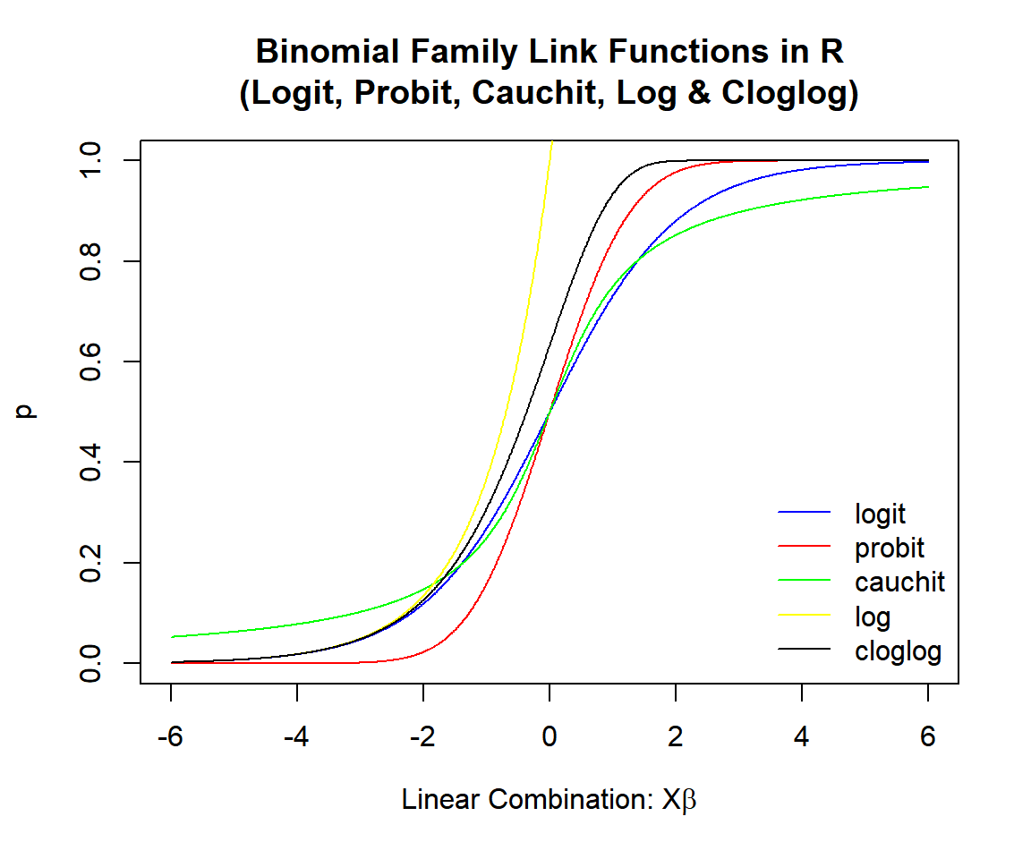
Binomial Family Link Functions in R (Logit, Probit, Cauchit, Log & Cloglog)
| Distribution | Dependent Variable |
|---|---|
|
Bernoulli \((p)\): \(\{0, 1\}\) |
1’s & 0’s Or factor with two levels: like ‘Yes’ & ‘No’ |
|
Binomial \((n, p)\): \(\{0, 1, \ldots, n\}\) |
Matrix of counts of ‘success’ and counts of ‘failure’ from cases of ‘success’ or ‘failure’ |
|
Or vector of proportion of ‘success’ and number of cases as weights |
2 Logit Link in R
Link function:
\(\begin{align} \log\left(\frac{p}{1-p}\right) & = X\beta \\ & = \beta_0 + \beta_1 x_1 + \beta_2 x_2 + \cdots + \beta_m x_m. \end{align}\)
Parameter function:
\(p = \frac{\exp(X\beta)}{1 + \exp(X\beta)} = \frac{1}{1 + \exp(-X\beta)}.\)
Bernoulli with Two Levels (Example: 1’s and 0’s)
set.seed(123) # For replication

n = 100

# Simulate linear combination (with mean 0)

x1 = rnorm(n, mean = 10, sd = 1.5)
x2 = rnorm(n, mean = 15, sd = 1.25)
xb = 5 + 4*x1 - 3*x2 + rnorm(n, 0, 1.5)

# Derive logit Bernoulli 1's and 0's based on 0.5 threshold

p_logit = exp(xb)/(1+exp(xb))
y_logit = ifelse(p_logit >= 0.5, 1, 0)
# Run GLM for logit model with 1's and 0's
logit_model = glm(y_logit ~ x1 + x2, family = binomial())
summary(logit_model)
Call:
glm(formula = y_logit ~ x1 + x2, family = binomial())

Coefficients:
            Estimate Std. Error z value Pr(>|z|)
(Intercept)   5.4722     5.7079   0.959    0.338
x1            3.7335     0.8964   4.165 3.12e-05 ***
x2           -2.8339     0.7118  -3.982 6.85e-05 ***
---
Signif. codes:  0 '***' 0.001 '**' 0.01 '*' 0.05 '.' 0.1 ' ' 1

(Dispersion parameter for binomial family taken to be 1)

    Null deviance: 137.186  on 99  degrees of freedom
Residual deviance:  45.924  on 97  degrees of freedom
AIC: 51.924

Number of Fisher Scoring iterations: 7Model: \[\widehat p = \frac{\exp(5.4722 + 3.7335 x_1 - 2.8339 x_2)}{1 + \exp(5.4722 + 3.7335 x_1 - 2.8339 x_2)}.\]
# Check the actual vs. predicted probabilities

plot(p_logit, logit_model$fitted.values,
     ylab = "Fitted Probabilities",
     xlab = "Actual Probabilities",
     col = (y_logit + 2),
     main = "Logit Model: Plot of Actual versus Fitted Probabilities")
abline(v = 0.5, h = 0.5)
legend("topleft",
       c("0", "1"),
       fill = c("red", "green"))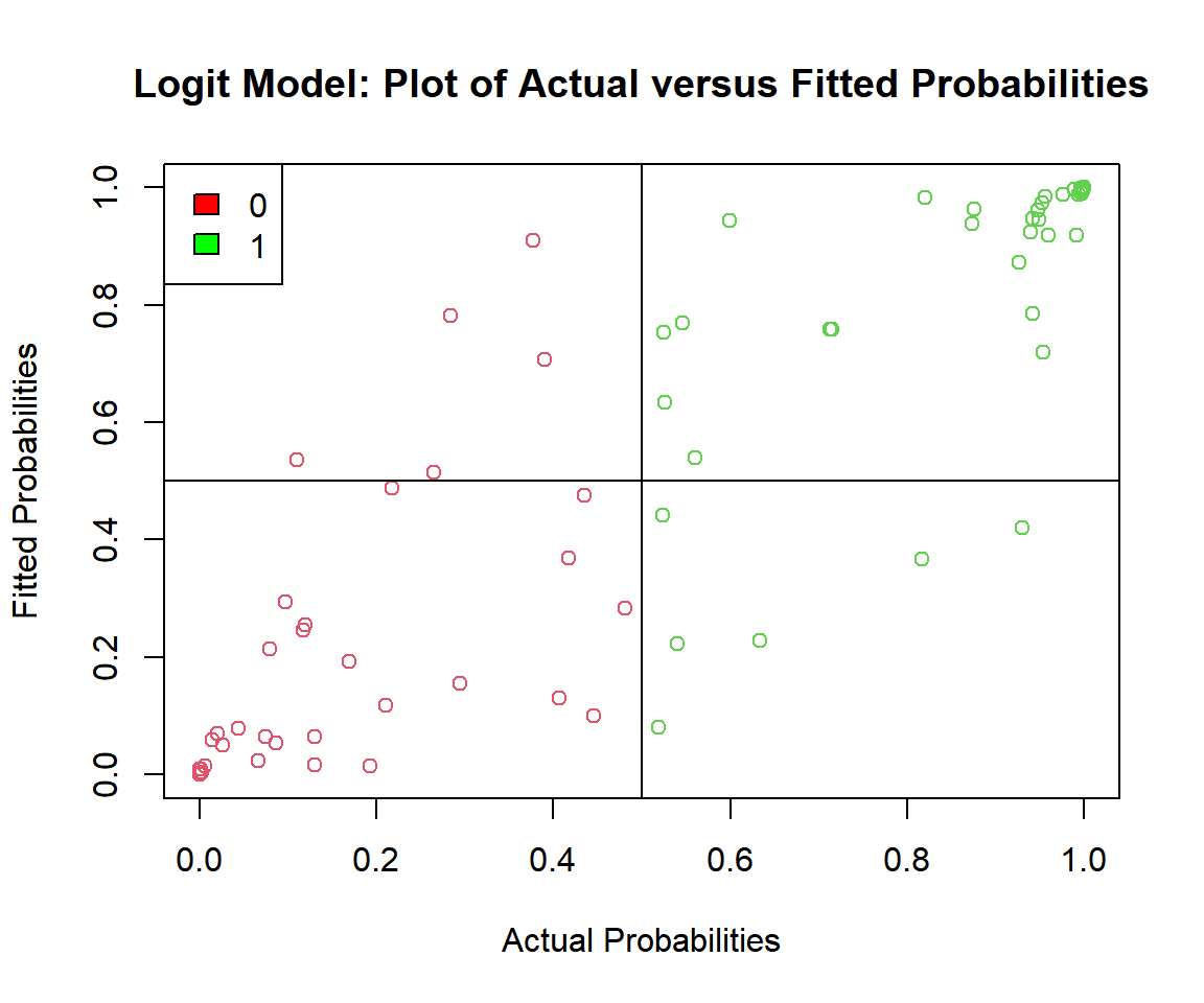
Logit Model: Plot of Actual versus Fitted Probabilities in R
# Check the actuals vs. the decision boundary

b0 = summary(logit_model)$coefficients[1,1]
b1 = summary(logit_model)$coefficients[2,1]
b2 = summary(logit_model)$coefficients[3,1]

plot(x1, x2, col = (y_logit + 2),
     main = "Logit Model: Plot of Actuals versus Decision Boundary")
segments(x0 = (-b0/b1 - (b2*min(x2))/b1), y0 = min(x2),
         x1 = (-b0/b1 - (b2*max(x2))/b1), y1 = max(x2),
         col = "blue")
legend("topleft",
       c("0", "1"),
       fill = c("red", "green"))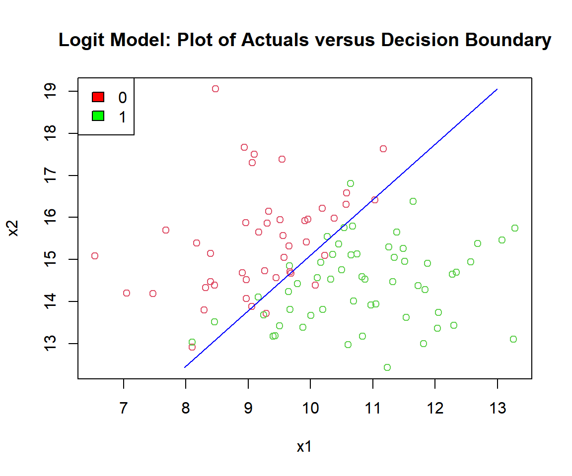
Logit Model: Plot of Logistic Regression Decision Boundary in R
| Actual \ Predicted | Positive (PP) | Negative (PN) | Total |
|---|---|---|---|
| Positive (P) |
True Positive 50 |
False Negative 6 |
56 |
| Negative (N) |
False Positive 5 |
True Negative 39 |
44 |
| Total | 55 | 45 | 100 |
Accuracy:
\(\frac{\text{True Positive } + \text{ True Negative}}{N} = 0.89\)
# Accuracy

true_positive = sum((p_logit>=0.5)*(logit_model$fitted.values>=0.5))
true_negaive = sum((p_logit<0.5)*(logit_model$fitted.values<0.5))
accuracy = (true_positive + true_negaive)/n
accuracy
[1] 0.89Binomial with Size N’s and Successes X’s
set.seed(123) # For replication

n = 1000

# Simulate linear combination (with mean 0)

x1 = rnorm(n, mean = 10, sd = 1.5)
x2 = rnorm(n, mean = 15, sd = 1.25)
xb = 5 + 4*x1 - 3*x2

# Simulate logit binomial with different size N's and successes X's

p_logit = exp(xb)/(1+exp(xb))
N = sample(10:30, n, replace = TRUE)
X = rbinom(n, size = N, prob = p_logit)
y_logit = cbind(X, N-X)
# Run GLM for logit model with successes and failures
logit_model = glm(y_logit ~ x1 + x2, family = binomial())
summary(logit_model)
Call:
glm(formula = y_logit ~ x1 + x2, family = binomial())

Coefficients:
            Estimate Std. Error z value Pr(>|z|)
(Intercept)  5.73752    0.42169   13.61   <2e-16 ***
x1           3.87544    0.06760   57.33   <2e-16 ***
x2          -2.96655    0.05465  -54.28   <2e-16 ***
---
Signif. codes:  0 '***' 0.001 '**' 0.01 '*' 0.05 '.' 0.1 ' ' 1

(Dispersion parameter for binomial family taken to be 1)

    Null deviance: 20574.57  on 999  degrees of freedom
Residual deviance:   649.72  on 997  degrees of freedom
AIC: 1746.2

Number of Fisher Scoring iterations: 6
Binomial with Proportion of Successes and Number of Cases as Weights
set.seed(123) # For replication

n = 1000

# Simulate linear combination (with mean 0)

x1 = rnorm(n, mean = 10, sd = 1.5)
x2 = rnorm(n, mean = 15, sd = 1.25)
xb = 5 + 4*x1 - 3*x2

# Simulate logit binomial with proportion of successes

p_logit = exp(xb)/(1+exp(xb))
cases = sample(20:50, n, replace = TRUE)
success = rbinom(n, size = cases, prob = p_logit)
y_logit = success/cases
# Run GLM for logit model with proportion of successes
logit_model = glm(y_logit ~ x1 + x2,
weights = cases, family = binomial())
summary(logit_model)
Call:
glm(formula = y_logit ~ x1 + x2, family = binomial(), weights = cases)

Coefficients:
            Estimate Std. Error z value Pr(>|z|)
(Intercept)  4.71521    0.32589   14.47   <2e-16 ***
x1           4.01229    0.05351   74.98   <2e-16 ***
x2          -2.98684    0.04234  -70.55   <2e-16 ***
---
Signif. codes:  0 '***' 0.001 '**' 0.01 '*' 0.05 '.' 0.1 ' ' 1

(Dispersion parameter for binomial family taken to be 1)

    Null deviance: 35688.17  on 999  degrees of freedom
Residual deviance:   622.22  on 997  degrees of freedom
AIC: 2022.9

Number of Fisher Scoring iterations: 6
3 Probit Link in R
Link function:
\(\begin{align} \Phi^{-1}(p) & = X\beta \\ & = \beta_0 + \beta_1 x_1 + \beta_2 x_2 + \cdots + \beta_m x_m. \end{align}\)
Parameter function:
\(p = \Phi(X\beta).\)
Where \(\Phi\) is the cumulative distribution function of the standard normal distribution.
set.seed(123) # For replication

n = 100

# Simulate linear combination (with mean 0)

x1 = rnorm(n, mean = 2, sd = 0.5)
x2 = rnorm(n, mean = 3, sd = 0.25)
xb = 5 + 2*x1 - 3*x2 + rnorm(n, 0, 1)

# Derive probit Bernoulli 1's and 0's based on 0.5 threshold

p_probit = pnorm(xb)
y_probit = ifelse(p_probit >= 0.5, 1, 0)
# Run GLM for probit model
probit_model = glm(y_probit ~ x1 + x2,
family = binomial(link = "probit"))
summary(probit_model)
Call:
glm(formula = y_probit ~ x1 + x2, family = binomial(link = "probit"))

Coefficients:
            Estimate Std. Error z value Pr(>|z|)
(Intercept)    6.783      2.288   2.964  0.00303 **
x1             1.893      0.441   4.292 1.77e-05 ***
x2            -3.458      0.823  -4.202 2.64e-05 ***
---
Signif. codes:  0 '***' 0.001 '**' 0.01 '*' 0.05 '.' 0.1 ' ' 1

(Dispersion parameter for binomial family taken to be 1)

    Null deviance: 134.602  on 99  degrees of freedom
Residual deviance:  90.707  on 97  degrees of freedom
AIC: 96.707

Number of Fisher Scoring iterations: 6Model: \[\widehat p = \Phi(6.783 + 1.893 x_1 - 3.458 x_2).\]
# Check the actual vs. predicted probabilities

plot(p_probit, probit_model$fitted.values,
     ylab = "Fitted Probabilities",
     xlab = "Actual Probabilities",
     col = (y_probit + 2),
     main = "Probit Model: Plot of Actual versus Fitted Probabilities")
abline(v = 0.5, h = 0.5)
legend("topleft",
       c("0", "1"),
       fill = c("red", "green"))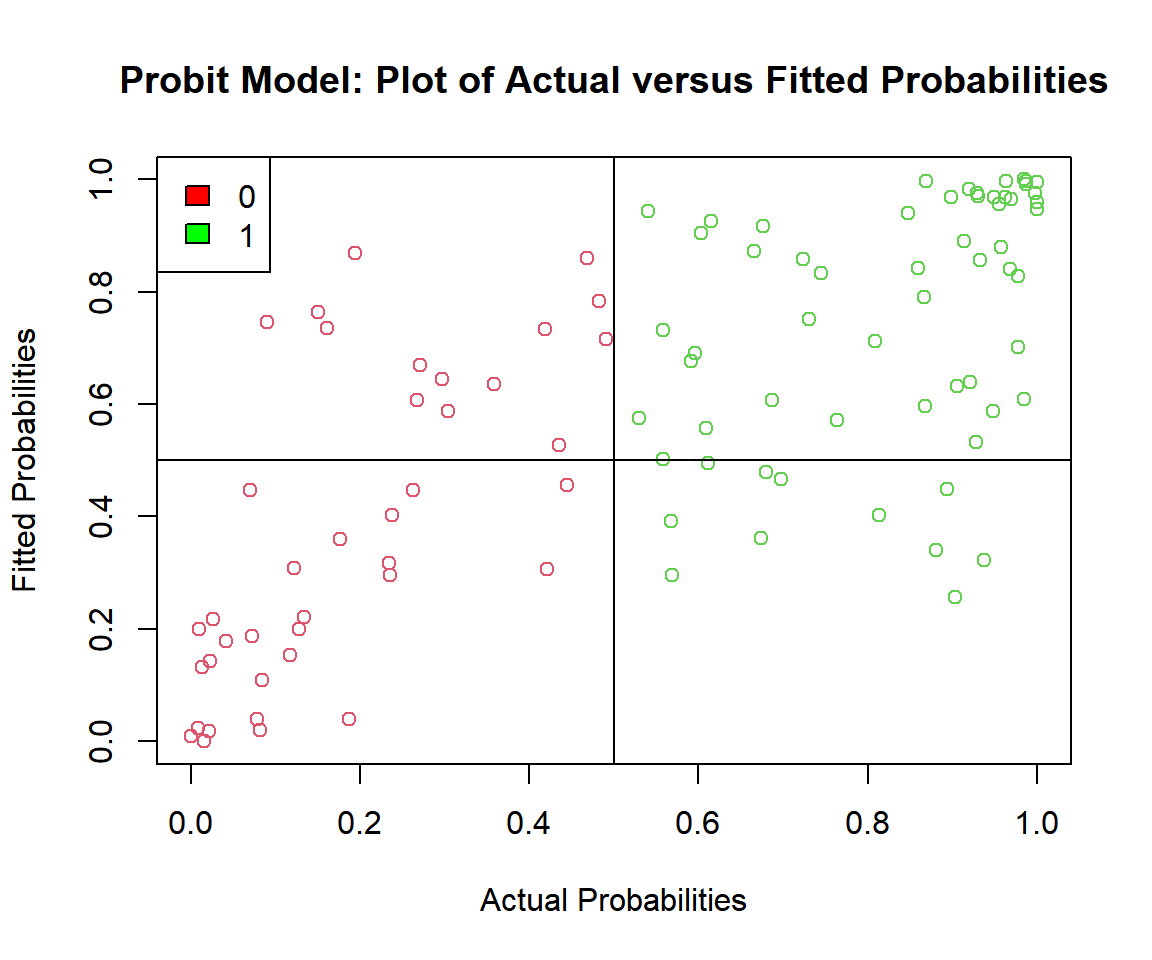
Probit Model: Plot of Actual versus Fitted Probabilities in R
# Check the actuals vs. the decision boundary

b0 = summary(probit_model)$coefficients[1,1]
b1 = summary(probit_model)$coefficients[2,1]
b2 = summary(probit_model)$coefficients[3,1]

plot(x1, x2, col = (y_probit + 2),
     main = "Probit Model: Plot of Actuals versus Decision Boundary")
segments(x0 = (-b0/b1 - (b2*min(x2))/b1), y0 = min(x2),
         x1 = (-b0/b1 - (b2*max(x2))/b1), y1 = max(x2),
         col = "blue")
legend("topleft",
       c("0", "1"),
       fill = c("red", "green"))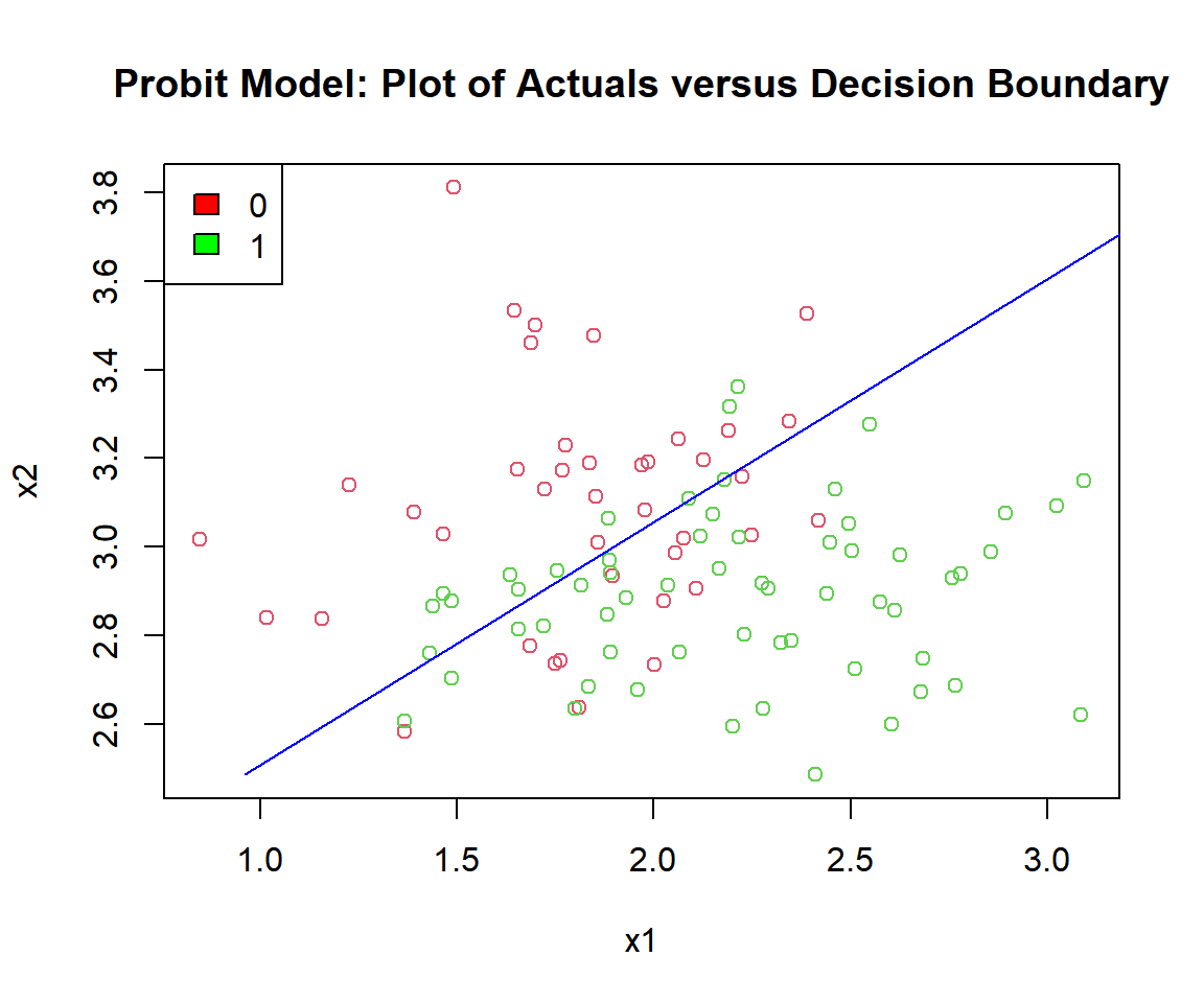
Probit Model: Plot of Logistic Regression Decision Boundary in R
| Actual \ Predicted | Positive (PP) | Negative (PN) | Total |
|---|---|---|---|
| Positive (P) |
True Positive 49 |
False Negative 11 |
60 |
| Negative (N) |
False Positive 14 |
True Negative 26 |
40 |
| Total | 63 | 37 | 100 |
Accuracy:
\(\frac{\text{True Positive } + \text{ True Negative}}{N} = 0.75\)
# Accuracy

true_positive = sum((p_probit>=0.5)*(probit_model$fitted.values>=0.5))
true_negaive = sum((p_probit<0.5)*(probit_model$fitted.values<0.5))
accuracy = (true_positive + true_negaive)/n
accuracy
[1] 0.754 Cauchit Link in R
Link function:
\(\begin{align} \tan(\pi(p-\frac{1}{2})) & = X\beta \\ & = \beta_0 + \beta_1 x_1 + \beta_2 x_2 + \cdots + \beta_m x_m. \end{align}\)
Parameter function:
\(p = \frac{1}{\pi}\arctan\left(X\beta\right) + \frac{1}{2}.\)
This is based on the cumulative distribution function of the standard Cauchy distribution.
set.seed(1234) # For replication

n = 100

# Simulate linear combination (with mean 0)

x1 = rnorm(n, mean = 2, sd = 0.5)
x2 = rnorm(n, mean = 3, sd = 0.25)
xb = 2 + 5*x1 - 4*x2 + rnorm(n, 0, 2.5)

# Derive cauchit Bernoulli 1's and 0's based on 0.5 threshold

p_cauchit = (1/pi)*atan(xb) + 0.5
y_cauchit = ifelse(p_cauchit >= 0.5, 1, 0)
# Run GLM for cauchit model
cauchit_model = glm(y_cauchit ~ x1 + x2,
family = binomial(link = "cauchit"))
summary(cauchit_model)
Call:
glm(formula = y_cauchit ~ x1 + x2, family = binomial(link = "cauchit"))

Coefficients:
            Estimate Std. Error z value Pr(>|z|)
(Intercept)    1.848      4.299   0.430  0.66735
x1             5.889      1.993   2.955  0.00312 **
x2            -4.226      1.984  -2.130  0.03313 *
---
Signif. codes:  0 '***' 0.001 '**' 0.01 '*' 0.05 '.' 0.1 ' ' 1

(Dispersion parameter for binomial family taken to be 1)

    Null deviance: 138.589  on 99  degrees of freedom
Residual deviance:  85.704  on 97  degrees of freedom
AIC: 91.704

Number of Fisher Scoring iterations: 11Model: \[\widehat p = \frac{1}{\pi}\arctan\left(1.848 + 5.889 x_1 - 4.226 x_2\right) + \frac{1}{2}.\]
# Check the actual vs. predicted probabilities

plot(p_cauchit, cauchit_model$fitted.values,
     ylab = "Fitted Probabilities",
     xlab = "Actual Probabilities",
     col = (y_cauchit + 2),
     main = "Cauchit Model: Plot of Actual versus Fitted Probabilities")
abline(v = 0.5, h = 0.5)
legend("topleft",
       c("0", "1"),
       fill = c("red", "green"))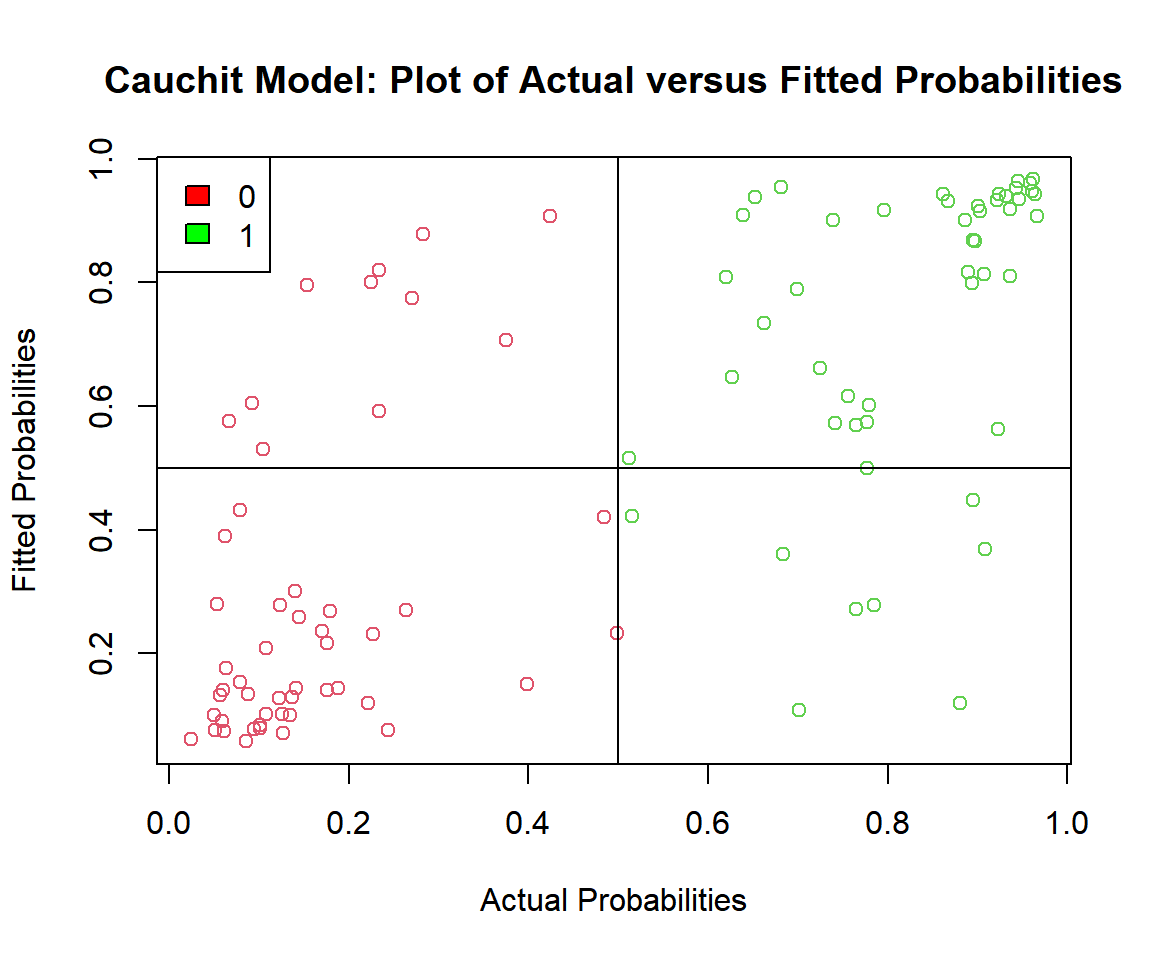
Cauchit Model: Plot of Actual versus Fitted Probabilities in R
# Check the actuals vs. the decision boundary

b0 = summary(cauchit_model)$coefficients[1,1]
b1 = summary(cauchit_model)$coefficients[2,1]
b2 = summary(cauchit_model)$coefficients[3,1]

plot(x1, x2, col = (y_cauchit + 2),
     main = "Cauchit Model: Plot of Actuals versus Decision Boundary")
segments(x0 = (-b0/b1 - (b2*min(x2))/b1), y0 = min(x2),
         x1 = (-b0/b1 - (b2*max(x2))/b1), y1 = max(x2),
         col = "blue")
legend("topleft",
       c("0", "1"),
       fill = c("red", "green"))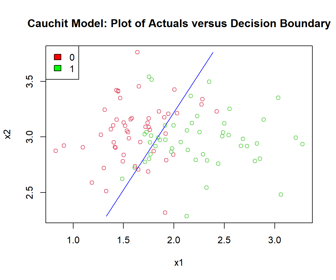
Cauchit Model: Plot of Logistic Regression Decision Boundary in R
| Actual \ Predicted | Positive (PP) | Negative (PN) | Total |
|---|---|---|---|
| Positive (P) |
True Positive 40 |
False Negative 9 |
49 |
| Negative (N) |
False Positive 11 |
True Negative 40 |
51 |
| Total | 51 | 49 | 100 |
Accuracy:
\(\frac{\text{True Positive } + \text{ True Negative}}{N} = 0.8\)
# Accuracy

true_positive = sum((p_cauchit>=0.5)*(cauchit_model$fitted.values>=0.5))
true_negaive = sum((p_cauchit<0.5)*(cauchit_model$fitted.values<0.5))
accuracy = (true_positive + true_negaive)/n
accuracy
[1] 0.85 Log Link in R
Link function:
\(\begin{align} \log(p) & = X\beta \\ & = \beta_0 + \beta_1 x_1 + \beta_2 x_2 + \cdots + \beta_m x_m. \end{align}\)
Parameter function:
\(p = \exp(X\beta).\)
set.seed(123) # For replication

n = 100

# Simulate linear combination (with max value less than 0)

x1 = runif(n, 0, 1)
x2 = rexp(n, 10)
xb = 0.1 - x1 - x2 + rnorm(n, 0, 0.2)

# Derive log Bernoulli 1's and 0's based on 0.5 threshold

p_log = exp(xb)
y_log = ifelse(p_log >= 0.5, 1, 0)
# Run GLM for log model with valid guess start value for xb < 0 for all values
log_model = glm(y_log ~ x1 + x2,
family = binomial(link = "log"),
start = c(-1, -1, -1))
summary(log_model)
Call:
glm(formula = y_log ~ x1 + x2, family = binomial(link = "log"),
    start = c(-1, -1, -1))

Coefficients:
            Estimate Std. Error z value Pr(>|z|)
(Intercept)  0.03319    0.04167   0.796    0.426
x1          -1.06287    0.19178  -5.542 2.99e-08 ***
x2          -0.71202    0.91310  -0.780    0.436
---
Signif. codes:  0 '***' 0.001 '**' 0.01 '*' 0.05 '.' 0.1 ' ' 1

(Dispersion parameter for binomial family taken to be 1)

    Null deviance: 123.820  on 99  degrees of freedom
Residual deviance:  91.739  on 97  degrees of freedom
AIC: 97.739

Number of Fisher Scoring iterations: 25Model: \[\widehat p = \exp(0.03319 - 1.06287 x_1 - 0.71202 x_2).\]
# Check the actual vs. predicted probabilities

plot(p_log, log_model$fitted.values,
     ylab = "Fitted Probabilities",
     xlab = "Actual Probabilities",
     col = (y_log + 2),
     main = "Log Model: Plot of Actual versus Fitted Probabilities")
abline(v = 0.5, h = 0.5)
legend("topleft",
       c("0", "1"),
       fill = c("red", "green"))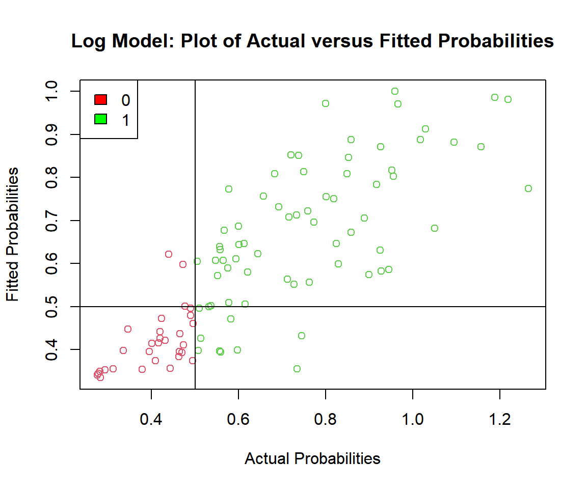
Log Model: Plot of Actual versus Fitted Probabilities in R
# Check the actuals vs. the decision boundary

b0 = summary(log_model)$coefficients[1,1]
b1 = summary(log_model)$coefficients[2,1]
b2 = summary(log_model)$coefficients[3,1]
c = log(1/2)

plot(x1, x2, col = (y_log + 2),
     main = "Log Model: Plot of Actuals versus Decision Boundary")
segments(x0 = (c/b1 - b0/b1 - (b2*min(x2))/b1), y0 = min(x2),
         x1 = (c/b1 - b0/b1 - (b2*max(x2))/b1), y1 = max(x2),
         col = "blue")
legend("topleft",
       c("0", "1"),
       fill = c("red", "green"))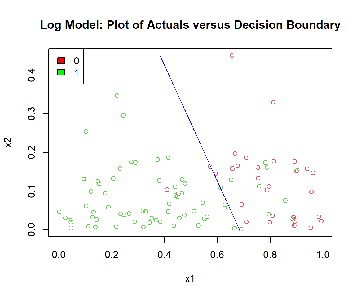
Log Model: Plot of Logistic Regression Decision Boundary in R
| Actual \ Predicted | Positive (PP) | Negative (PN) | Total |
|---|---|---|---|
| Positive (P) |
True Positive 59 |
False Negative 10 |
69 |
| Negative (N) |
False Positive 3 |
True Negative 28 |
31 |
| Total | 62 | 38 | 100 |
Accuracy:
\(\frac{\text{True Positive } + \text{ True Negative}}{N} = 0.87\)
# Accuracy

true_positive = sum((p_log>=0.5)*(log_model$fitted.values>=0.5))
true_negaive = sum((p_log<0.5)*(log_model$fitted.values<0.5))
accuracy = (true_positive + true_negaive)/n
accuracy
[1] 0.876 Complementary Log-Log Link in R
Link function:
\(\begin{align} \log(-\log(1-p)) & = X\beta \\ & = \beta_0 + \beta_1 x_1 + \beta_2 x_2 + \cdots + \beta_m x_m. \end{align}\)
Parameter function:
\(p = 1-\exp(-\exp(X\beta)).\)
set.seed(123) # For replication

n = 100

# Simulate linear combination

x1 = rnorm(n, mean = 5, sd = 0.25)
x2 = rnorm(n, mean = 7, sd = 0.25)
xb = 2.7 + 5*x1 - 4*x2 + rnorm(n, 0, 1.2)

# Derive cloglog Bernoulli 1's and 0's based on 0.5 threshold

p_cloglog = 1-exp(-exp(xb))
y_cloglog = ifelse(p_cloglog >= 0.5, 1, 0)
# Run GLM for cloglog model
cloglog_model = glm(y_cloglog ~ x1 + x2,
family = binomial(link = "cloglog"))
summary(cloglog_model)
Call:
glm(formula = y_cloglog ~ x1 + x2, family = binomial(link = "cloglog"))

Coefficients:
            Estimate Std. Error z value Pr(>|z|)
(Intercept)   3.6496     6.5269   0.559    0.576
x1            4.7164     1.1349   4.156 3.24e-05 ***
x2           -3.9050     0.9784  -3.991 6.57e-05 ***
---
Signif. codes:  0 '***' 0.001 '**' 0.01 '*' 0.05 '.' 0.1 ' ' 1

(Dispersion parameter for binomial family taken to be 1)

    Null deviance: 131.791  on 99  degrees of freedom
Residual deviance:  82.724  on 97  degrees of freedom
AIC: 88.724

Number of Fisher Scoring iterations: 8Model: \[\widehat p = 1-\exp(-\exp(3.6496 + 4.7164 x_1 - 3.9050 x_2)).\]
# Check the actual vs. predicted probabilities

plot(p_cloglog, cloglog_model$fitted.values,
     ylab = "Fitted Probabilities",
     xlab = "Actual Probabilities",
     col = (y_cloglog + 2),
     main = "Cloglog Model: Plot of Actual versus Fitted Probabilities")
abline(v = 0.5, h = 0.5)
legend("topleft",
       c("0", "1"),
       fill = c("red", "green"))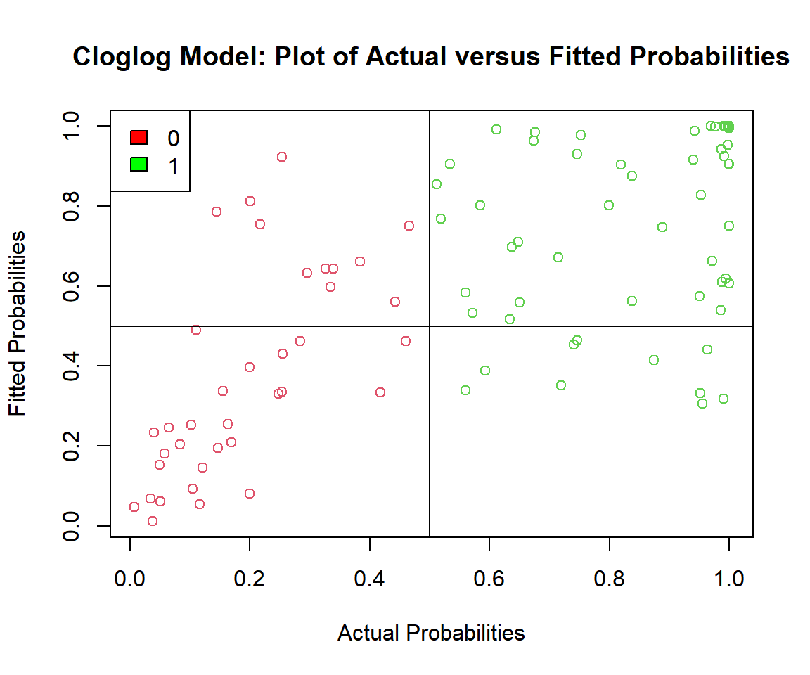
Cloglog Model: Plot of Actual versus Fitted Probabilities in R
# Check the actuals vs. the decision boundary

b0 = summary(cloglog_model)$coefficients[1,1]
b1 = summary(cloglog_model)$coefficients[2,1]
b2 = summary(cloglog_model)$coefficients[3,1]
c = log(-log(1/2))

plot(x1, x2, col = (y_cloglog + 2),
     main = "Cloglog Model: Plot of Actuals versus Decision Boundary")
segments(x0 = (c/b1 - b0/b1 - (b2*min(x2))/b1), y0 = min(x2),
         x1 = (c/b1 - b0/b1 - (b2*max(x2))/b1), y1 = max(x2),
         col = "blue")
legend("topleft",
       c("0", "1"),
       fill = c("red", "green"))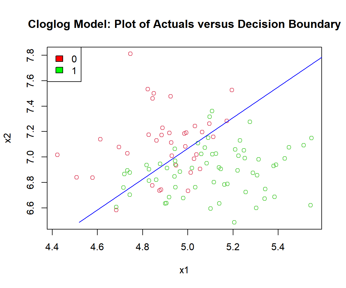
Cloglog Model: Plot of Logistic Regression Decision Boundary in R
| Actual \ Predicted | Positive (PP) | Negative (PN) | Total |
|---|---|---|---|
| Positive (P) |
True Positive 53 |
False Negative 10 |
63 |
| Negative (N) |
False Positive 11 |
True Negative 26 |
37 |
| Total | 64 | 36 | 100 |
Accuracy:
\(\frac{\text{True Positive } + \text{ True Negative}}{N} = 0.79\)
# Accuracy

true_positive = sum((p_cloglog>=0.5)*(cloglog_model$fitted.values>=0.5))
true_negaive = sum((p_cloglog<0.5)*(cloglog_model$fitted.values<0.5))
accuracy = (true_positive + true_negaive)/n
accuracy
[1] 0.79The feedback form is a Google form but it does not collect any personal information.
Please click on the link below to go to the Google form.
Thank You!
Go to Feedback Form
Copyright © 2020 - 2026. All Rights Reserved by Stats Codes