Multiple Linear Regression in R
Here, we discuss multiple linear regression in R with interpretations, including variable selection, diagnostic tests and prediction.
Multiple linear regression (or ordinary least squares) in R can be
performed with the lm() function from the "stats" package in the base
version of R.
Multiple linear regression can be used to study the linear relationships, if they exist, between a dependent variable \((y)\) and a set of independent variables \((x_1, x_2, \ldots, x_p)\).
For single independent variable, see simple linear regression.
The multiple linear regression framework is based on the theoretical assumption that: \[y = \beta_0 + \beta_1 x_1 + \beta_2 x_2 + \cdots + \beta_p x_p + \varepsilon,\]
where \(\varepsilon\) represents the error terms that are 1) independent, 2) normal distributed, 3) have constant variance, and 4) have mean zero.
The multiple linear regression model estimates the true coefficients,
\(\beta_1, \beta_2, \ldots, \beta_p\),
as \(\widehat \beta_1, \widehat \beta_2,
\ldots, \widehat \beta_p\), and the true intercept, \(\beta_0\), as \(\widehat \beta_0\).
Then for any \(x_1, x_2, \ldots, x_p\) values, these are
used to predict or estimate the true \(y\), as \(\widehat y\), with the equation below:
\[\widehat y = \widehat \beta_0 + \widehat \beta_1 x_1 + \widehat \beta_2 x_2 + \cdots + \widehat \beta_p x_p.\]
Sample Steps to Run a Multiple Regression Model:
# Create the data samples for the regression model
# Values are matched based on matching position in each sample

y = c(3.7, 1.4, 0.6, 5.2, 1.7, 8.2, 1.8, 0.9)
x1 = c(4.4, 1.9, 3.1, 4.2, 3.2, 3.4, 3.2, 4.2)
x2 = c(7.0, 5.4, 6.9, 5.4, 7.1, 4.0, 7.5, 8.1)
x3 = c(5.1, 4.6, 4.2, 3.7, 5.7, 5.5, 6.6, 4.7)
df_data = data.frame(y, x1, x2, x3)
df_data

# Run the multiple regression model

model = lm(y ~ x1 + x2 + x3)
summary(model)

#or

model = lm(y ~ x1 + x2 + x3, data = df_data)
summary(model)

#or

model = lm(y ~ ., data = df_data)
summary(model)
y x1 x2 x3
1 3.7 4.4 7.0 5.1
2 1.4 1.9 5.4 4.6
3 0.6 3.1 6.9 4.2
4 5.2 4.2 5.4 3.7
5 1.7 3.2 7.1 5.7
6 8.2 3.4 4.0 5.5
7 1.8 3.2 7.5 6.6
8 0.9 4.2 8.1 4.7
Call:
lm(formula = y ~ x1 + x2 + x3)

Residuals:
       1        2        3        4        5        6        7        8
-0.09364 -0.05803  0.08221 -0.04665 -0.04157  0.07984  0.00200  0.07583

Coefficients:
            Estimate Std. Error t value Pr(>|t|)
(Intercept)  4.00872    0.27660   14.49 0.000132 ***
x1           2.01759    0.04613   43.74 1.63e-06 ***
x2          -1.98851    0.02807  -70.85 2.38e-07 ***
x3           0.94648    0.04051   23.37 1.99e-05 ***
---
Signif. codes:  0 '***' 0.001 '**' 0.01 '*' 0.05 '.' 0.1 ' ' 1

Residual standard error: 0.09345 on 4 degrees of freedom
Multiple R-squared:  0.9993,    Adjusted R-squared:  0.9987
F-statistic: 1839 on 3 and 4 DF, p-value: 9.844e-07| Argument | Usage |
| y ~ x1 + x2 +…+ xp | y is the dependent sample, and x1, x2, …, xp are the independent samples |
| y ~ ., data | y is the dependent sample, and "." means all other variables are in the model |
| data | The dataframe object that contains the dependent and independent variables |
Creating Multiple Regression Summary Object and Model Object:
# Create data
x1 = rnorm(50, 2, 2)
x2 = rnorm(50, 4, 1)
x3 = rnorm(50, 3, 5)
y = 10 + 3*x1 + 5*x2 + x3 + rnorm(50, 0, 1)

# Create multiple regression summary and model objects
reg_summary = summary(lm(y ~ x1 + x2 + x3))
reg_model = lm(y ~ x1 + x2 + x3) Estimate Std. Error t value Pr(>|t|)
(Intercept) 10.5878090 0.71064298 14.89891 3.194497e-19
x1 3.0178477 0.09632893 31.32857 1.122980e-32
x2 4.9173301 0.16631105 29.56707 1.421922e-31
x3 0.9346396 0.04017148 23.26625 4.410456e-27(Intercept) x1 x2 x3
10.5878090 3.0178477 4.9173301 0.9346396 (Intercept) x1 x2 x3
10.5878090 3.0178477 4.9173301 0.9346396 There are more examples in the table below.
| Regression Component | Usage |
| reg_summary$coefficients | The estimated intercept and beta values: their standard error, t-value and p-value |
| reg_summary$residuals | The regression model residuals |
| reg_summary$r.squared | The model r-squared value |
| reg_summary$adj.r.squared | The model adjusted r-squared value |
| reg_summary$fstatistic | The f-statistic and the degrees of freedom |
| reg_summary$sigma | The model residuals standard error |
| reg_model$coefficients | The estimated intercept and beta values |
| reg_model$residuals | The regression model residuals |
| reg_model$fitted.values | The predicted y values |
| reg_model$df.residual | The degrees of freedom of the residuals |
| reg_model$model | The model dataframe |
1 Steps to Running a Multiple Regression in R
Using the "attitude" data from the "datasets" package with 10 sample rows from 30 rows below:
   rating complaints privileges learning raises critical advance
1      43         51         30       39     61       92      45
6      43         55         49       44     54       49      34
10     67         61         45       47     62       80      41
13     69         62         57       42     55       63      25
16     81         90         50       72     60       54      36
17     74         85         64       69     79       79      63
23     53         66         52       50     63       80      37
27     78         75         58       74     80       78      49
29     85         85         71       71     77       74      55
30     82         82         39       59     64       78      39
NOTE: The dependent variable is "rating".
The data is from a survey of employees. They are the percent of favorable responses to seven questions in each of 30 departments.
The goal is to be able predict the overall rating received from the employees using other responses to the survey questions, hence, the dependent variable is "rating". The predictors or independent variables are the other column variables which are also part of the responses to the survey questions.
1.1 Check the Dependent and Independent Variables for Linear Correlation
First, we can use the cor() function from the "stats"
package in the base version of R to check for linear correlation between
the dependent variable ("rating") and the independent variables, and
among the independent variables. The function produces a matrix of Pearson’s correlation
coefficients between every possible pair.
              rating complaints privileges  learning    raises  critical
rating     1.0000000  0.8254176  0.4261169 0.6236782 0.5901390 0.1564392
complaints 0.8254176  1.0000000  0.5582882 0.5967358 0.6691975 0.1877143
privileges 0.4261169  0.5582882  1.0000000 0.4933310 0.4454779 0.1472331
learning   0.6236782  0.5967358  0.4933310 1.0000000 0.6403144 0.1159652
raises     0.5901390  0.6691975  0.4454779 0.6403144 1.0000000 0.3768830
critical   0.1564392  0.1877143  0.1472331 0.1159652 0.3768830 1.0000000
advance    0.1550863  0.2245796  0.3432934 0.5316198 0.5741862 0.2833432
             advance
rating     0.1550863
complaints 0.2245796
privileges 0.3432934
learning   0.5316198
raises     0.5741862
critical   0.2833432
advance    1.0000000
The first row shows the results for the linear relationship between the dependent variable ("rating") and the independent variables. The results suggest a strong linear relationship between "rating" and some of the independent variables, particularly, "complaints" (0.83), "learning" (0.62), and "raises" (0.59).
We can also use the plot() function to visually check
for linear correlations based on the scatter plots of
all the variable pairs.
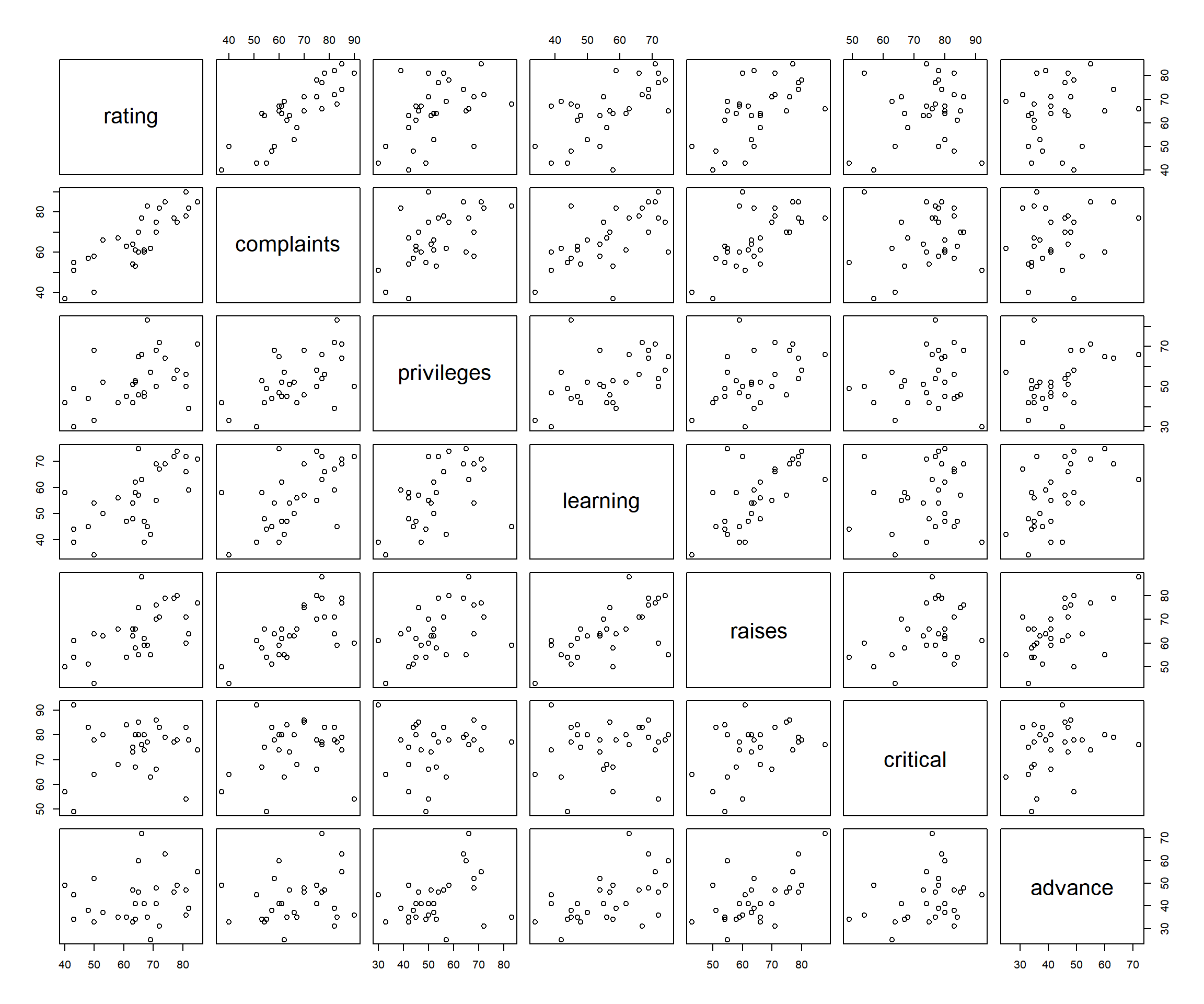
Scatter Plots of All Variable Pairs in R
The first row shows the scatter plots of the dependent variable ("rating") versus the independent variables. The results also suggest a strong linear relationship between "rating" and the variables "complaints", "learning", and "raises" which are the first, third, and fourth plots on the first row respectively. Hence, these three variables are candidates in the final model.
1.2 Perform Variable Selection
We could include some of the most correlated variables with "rating" in the model and remove or add variables based on whether they are significant. Alternatively, we could automate the variable selection process by using stepwise regression.
The step() function from the base "stats" package can be
used to perform various stepwise regression based on AIC.
Forward Stepwise Regression
Without any special preference for some variables, we can use the forward stepwise regression starting with no variable.
First, we set the intercept model and the full model. The intercept model has no variable in the model, while the full model contains all the variables available.
# Specify the intercept model
intercept_model = lm(rating ~ 1, data = attitude)

# Specify the full model
full_model = lm(rating ~ ., data = attitude)
#or
full_model = lm(rating ~ complaints + privileges + learning +
                raises + critical + advance, data = attitude)
Our variable selection then starts from the intercept (or null)
model. Then from the intercept model, based on AIC, we add one variable
repeatedly, until no other variable based on the AIC criterion
significantly improves model performance when added. Potentially, we can
pick variables up to the full set of variables available (or scope) if
they all significantly add to the predictive power of the model. Set
trace = 1 to see the steps of variable additions, it is set
to 0 here.
# Perform forward stepwise regression
step(intercept_model, direction = 'forward',
     scope = formula(full_model), trace = 0)
Call:
lm(formula = rating ~ complaints + learning, data = attitude)

Coefficients:
(Intercept)   complaints     learning
     9.8709       0.6435       0.2112
As can be seen above, the final selection includes only "complaints" and "learning". This means that other variables such as "raises" are not significantly increasing the predictive power of the model when added to the two, and these two are most likely the most predictive pair.
1.3 Run the Regression Model with the Chosen Variables
Run the multiple linear regression model using the lm()
function, and print the results using the summary()
function.
Call:
lm(formula = rating ~ complaints + learning, data = attitude)

Residuals:
     Min       1Q   Median       3Q      Max
-11.5568  -5.7331   0.6701   6.5341  10.3610

Coefficients:
            Estimate Std. Error t value Pr(>|t|)
(Intercept)   9.8709     7.0612   1.398    0.174
complaints    0.6435     0.1185   5.432 9.57e-06 ***
learning      0.2112     0.1344   1.571    0.128
---
Signif. codes:  0 '***' 0.001 '**' 0.01 '*' 0.05 '.' 0.1 ' ' 1

Residual standard error: 6.817 on 27 degrees of freedom
Multiple R-squared:  0.708, Adjusted R-squared:  0.6864
F-statistic: 32.74 on 2 and 27 DF,  p-value: 6.058e-08
Interpretation of the Results
- Coefficients:
- The estimated intercept (\(\widehat \beta_0\)) is \(\text{summary(model)\$coefficients[1, 1]}\) \(= 9.871\).
- The estimated coefficient for "complaints" or \(x_1\) (\(\widehat \beta_1\)) is \(\text{summary(model)\$coefficients[2, 1]}\) \(= 0.644\).
- The estimated coefficient for "learning" or \(x_2\) (\(\widehat \beta_2\)) is \(\text{summary(model)\$coefficients[3, 1]}\) \(= 0.211\).
- P-values:
For level of significance, \(\alpha = 0.05\).- The p-value for "complaints" is \(\text{summary(model)\$coefficients[2, 4]}\)
\(= 9.57\times 10^{-6}\).
Since the p-value is less than \(0.05\), we say that "complaints" is a statistically significant predictor of "rating". - The p-value for "learning" is \(\text{summary(model)\$coefficients[3, 4]}\)
\(= 0.128\).
Since the p-value is greater than \(0.05\), we say that "learning" is NOT a statistically significant predictor of "rating" in the presence of "complaints". However, this variable was included in the model because it increases the predictive power of the model when added to the "complaints" variable and passes the AIC criterion. - Remember that "learning" is highly correlated with "rating", with correlation of \(0.6236782\). Hence, when it is the only variable in the model the p-value is as low as \(0.000231\). Also, the r-squared is as high as \(0.389\) (or \(0.6236782^2\)). This means while "learning" is not statistically significant in the presence of "complaints", it is a useful predictor when added as a second variable as supported by the AIC criterion.
- The p-value for "complaints" is \(\text{summary(model)\$coefficients[2, 4]}\)
\(= 9.57\times 10^{-6}\).
- R-squared:
The r-squared value is \(\text{summary(model)\$r.squared}\) \(= 0.708\).
This means that the model, using the independent variables, "complaints" and "learning", explains \(70.8\%\) of the variations in the dependent variable \(y\) (rating) from the sample mean of \(y\), \(\bar y\).
1.4 Run the Regression Model Diagnostics
R allows you to plot standard regression diagnostics plots as below, and our focus here will be on the first two plots:
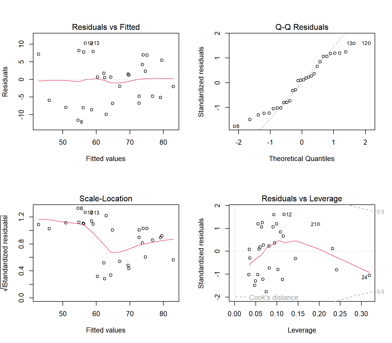
Standard Linear Regression Diagnostics Plots in R
The multiple linear regression framework has the theoretical assumption that the error terms (or residuals) are 1) independent, 2) normal distributed, 3) have constant variance, and 4) have mean zero.
By construction of the ordinary least squares model, the error terms have mean zero. Hence, we only need to check for 1) independence, 2) normal distribution, and 3) constant variance of the residuals.
Check for Independence and Constant Variance of Residuals
To check for independence and constant variance of the residuals, we can:
Look at the scatter plot of the residuals versus the fitted values and confirm that the residuals do not oscillate around zero in any noticeable or clear pattern. The plot of the residuals versus the fitted values below (or above) shows no pattern, hence, there is no evidence auto-correlation and they are independent.
Look at the scatter plot of the residuals versus the fitted values and confirm that the residuals do not depend on the predicted values. That is, the residuals do not increase (widen) or decrease (narrow) as the predicted value increases or decreases. The plot of the residuals versus the fitted values below (or above) does not show any widening or narrowing of the residuals, hence, there is no heteroskedasticity, and the constant variance assumption of residuals is not violated.
Look at the autocorrelation plot from the
acf()function in the base "stats" package. If the vertical lines, excluding the first one, are between the two blue horizontal lines, we can conclude that the residuals are not auto-correlated. All the lines are between the blue lines, this is another evidence of independence of residuals.
plot(model$fitted.values, model$residuals,
     main = "Residuals versus Fitted Values")
abline(h=0)

acf(model$residuals)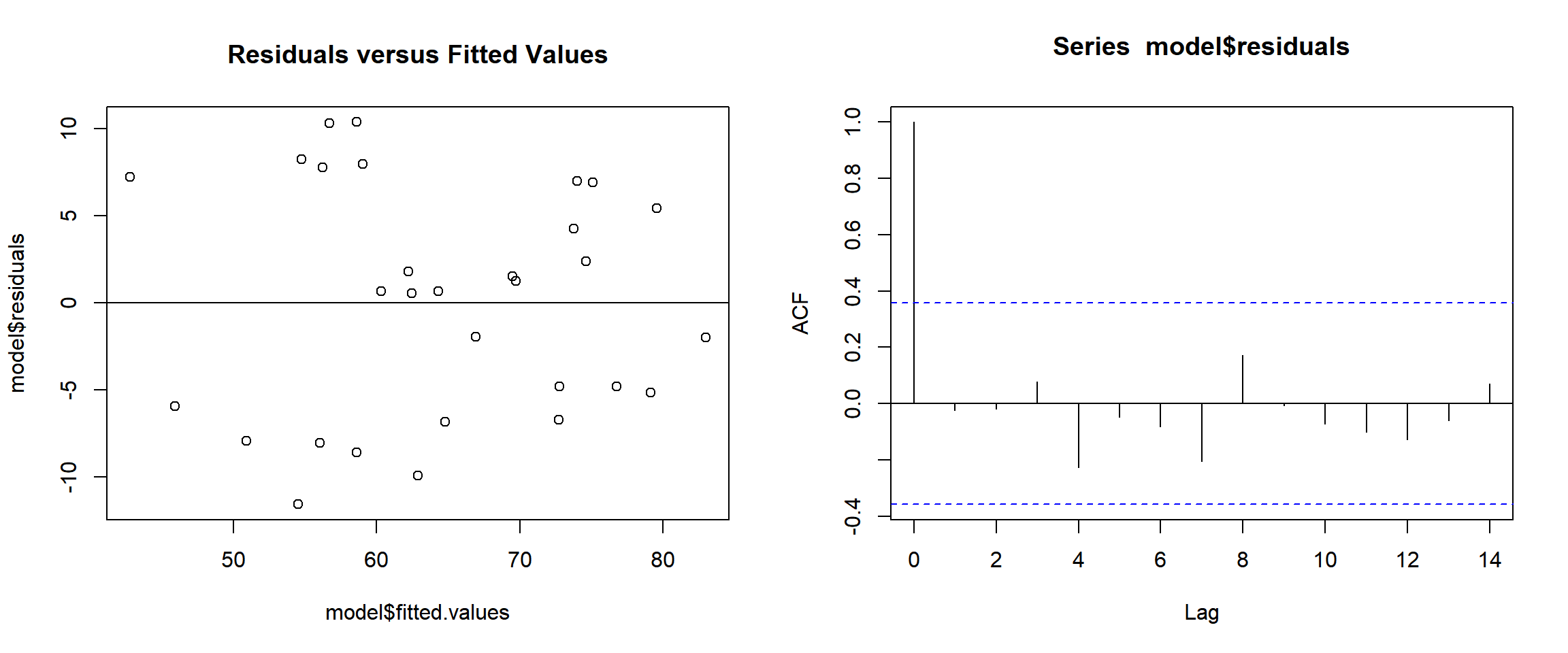
Regression Residual versus Fitted Values and Auto-correlation Plot in R
Check for Normality of the Residuals
Here we check for the normality of the residuals.
Normal Q-Q Plot
To check for the normality of the residuals, we can look at the quantile-quantile plot of the residuals versus the theoretical quantiles of from the standard normal distribution, and confirm that there is an alignment between the two.
If the values of the residuals are close to the theoretical values from normal distribution, the residuals will be very close to the quantile-quantile line on the plot. The closer they are to the line, the more the residuals fit to a normal distribution.
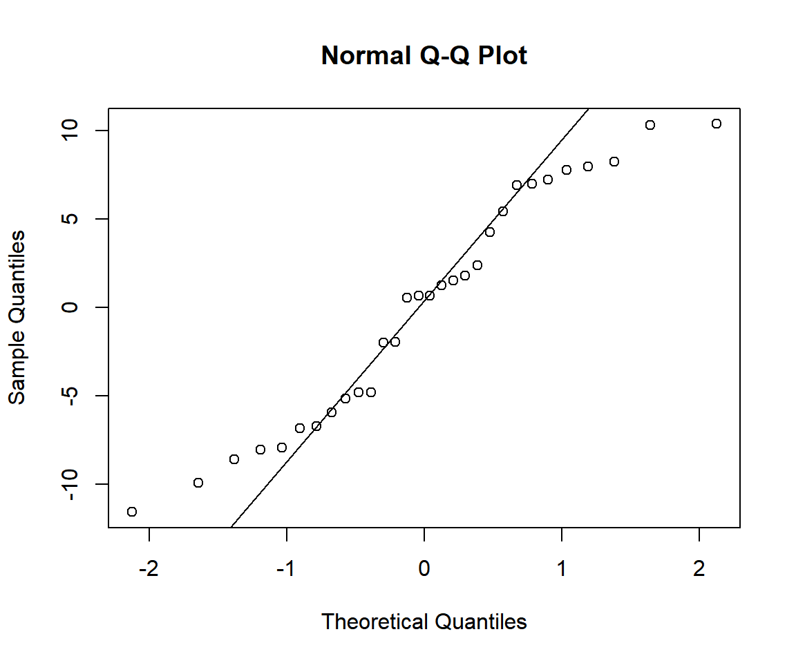
Quantile versus Quantile Plot of Regression Residuals in R
The result suggests that the residuals, given the sample size, fairly fit to a normal distribution as the dots are close to the diagonal except for about two values on the left tail and two values on the right tail.
Shapiro-Wilk Test
We can also use the Shapiro-Wilk test via the
shapiro.test() function from the base "stats" package. At
\(\alpha = 0.05\), that is, \(5\%\) level of significance, we reject the
null hypothesis that the residuals are normal distributed, if the
p-value is less than \(0.05\). Else, we
fail to reject that they are normal distributed.
    Shapiro-Wilk normality test

data:  model$residuals
W = 0.94486, p-value = 0.123
With the p-value \(0.123\) being greater than \(0.05\), we fail to reject the normal distribution assumption. Hence, our residuals are in line with the normal distribution assumption.
1.5 Use the Model for Prediction
To perform predictions, we can use the predict.lm()
function from the base "stats" package, or calculate directly.
Calculate Predictions Directly
For complaints = 70 (\(x_1 = 70\)), and learning = 60 (\(x_2 = 60\)).
#Set the coefficient and intercept
b0 = 9.8709; b1 = 0.6435; b2 = 0.2112

#or

b0 = model$coefficients[1]
b1 = model$coefficients[2]
b2 = model$coefficients[3]

prediction = b0 + b1*70 + b2*60
prediction
(Intercept)
67.58862 Use the predict.lm() Function for Prediction
For complaints = 70 (\(x_1 = 70\)), and learning = 60 (\(x_2 = 60\)).
       1
67.58862
For multiple values of both complaints and learning, for example, complaints = \(\{70, 60, 50\}\), and learning = \(\{60, 50, 45\}\).
complaints = c(70, 60, 50); learning = c(60, 50, 45)
pred_data = data.frame(complaints, learning)
pred_data
complaints learning
1 70 60
2 60 50
3 50 45 1 2 3
67.58862 59.04153 51.55039 We can also see the fitted values from the "attitude" data itself:
       1        2        3        4        5        6        7        8
50.92676 62.46037 69.48935 60.33851 74.00392 54.55679 64.81330 69.75025
       9       10       11       12       13       14       15       16
76.78918 59.05147 56.22644 56.71842 58.63903 72.78648 74.62755 82.99328
      17       18       19       20       21       22       23       24
79.14211 64.32132 66.95505 58.59926 42.79211 62.21935 62.90263 45.93016
      25       26       27       28       29       30
54.75804 72.72682 73.76290 56.05502 79.56450 75.09964
2 Extract Components from Regression Outputs in R
Here we show how to extract components from regression model objects and summary objects.
# Create multiple regression summary objects
reg_summary = summary(lm(rating ~ complaints + learning + advance,
                         data = attitude))

# Create multiple regression model objects
reg_model = lm(rating ~ complaints + learning + advance,
               data = attitude)
Extract Regression Model Coefficients
              Estimate Std. Error   t value     Pr(>|t|)
(Intercept) 13.5777411  7.5438997  1.799831 8.350310e-02
complaints   0.6227297  0.1181464  5.270830 1.646618e-05
learning     0.3123870  0.1541997  2.025859 5.315559e-02
advance -0.1869508 0.1448537 -1.290618 2.081957e-01(Intercept) complaints learning advance
13.5777411 0.6227297 0.3123870 -0.1869508 Extract Regression Model Residuals
           1            2            3            4            5            6
 -6.10726377   1.48534649   1.25011415   0.05137535   7.01848630 -12.21657656
           7            8            9           10           11           12
 -8.25102644   1.20122744  -7.77603263   8.41853970   5.65546524  11.54036528
          13           14           15           16           17           18
  8.36653187  -4.77844561   1.57994337  -4.38505144  -2.28656988   1.84649947
          19           20           21           22           23           24
 -1.37514374  -6.84352098   7.06128860   0.73273503 -10.38007320  -5.57659667
          25           26           27           28           29           30
  6.96965446  -1.74785274   3.76148134  -8.02661979   6.59304968   6.21866968
Extract Regression Model R-squared and Adjusted R-squared
[1] 0.725595[1] 0.6939329Extract Regression Model F-statistic and Degrees of Freedom
   value    numdf    dendf
22.91682  3.00000 26.00000
Extract Regression Model Residuals Standard Error
[1] 6.734267Extract Regression Model Fitted Values
       1        2        3        4        5        6        7        8
49.10726 61.51465 69.74989 60.94862 73.98151 55.21658 66.25103 69.79877
       9       10       11       12       13       14       15       16
79.77603 58.58146 58.34453 55.45963 60.63347 72.77845 75.42006 85.38505
      17       18       19       20       21       22       23       24
76.28657 63.15350 66.37514 56.84352 42.93871 63.26726 63.38007 45.57660
      25       26       27       28       29       30
56.03035 67.74785 74.23852 56.02662 78.40695 75.78133
Extract Regression Model Residuals’ Degrees of Freedom
[1] 26Extract Regression Model Data
  rating complaints learning advance
1     43         51       39      45
2     63         64       54      47
3     71         70       69      48
4     61         63       47      35
5     81         78       66      47
6 43 55 44 34The feedback form is a Google form but it does not collect any personal information.
Please click on the link below to go to the Google form.
Thank You!
Go to Feedback Form
Copyright © 2020 - 2026. All Rights Reserved by Stats Codes