1 Table of Beta Distribution Functions in R
2 Plot of Beta Distributions in R
3 Examples for Setting Parameters for Beta Distributions in R
4 rbeta(): Random Sampling from Beta Distributions in R
5 dbeta(): Probability Density Function for Beta Distributions in R
6 pbeta(): Cumulative Distribution Function for Beta Distributions in R
7 qbeta(): Derive Quantile for Beta Distributions in R

Here, we discuss beta distribution functions in R, plots, parameter setting, random sampling, density, cumulative distribution and quantiles.

The beta distribution with parameters \(\tt{shape\; 1}=\alpha\), and \(\tt{shape\; 2}=\beta\) has probability density function (pdf) formula as:

\[\begin{align} f(x) & = \frac{\Gamma(\alpha+\beta)}{\Gamma(\alpha)\Gamma(\beta)}\, x^{\alpha-1}(1-x)^{\beta-1} \\ & = \frac{1}{\operatorname{B}(\alpha,\beta)} x^{\alpha-1}(1-x)^{\beta-1},\end{align}\]

for \(x\in[0,1]\), where \(\alpha > 0\), and \(\beta > 0\).

\(\Gamma\) is the \(\tt{gamma\;function}\), and \(\mathrm{B}\) is the \(\tt{beta\;function}\).

The mean is \(\frac{\alpha}{\alpha + \beta}\), and the variance is \(\frac{\alpha\,\beta}{(\alpha + \beta)^2\,(\alpha + \beta+1)}\).

1 Table of Beta Distribution Functions in R

The table below shows the functions for beta distributions in R.

Table of Beta Distribution Functions in R
Function	Usage
rbeta(n, shape1, shape2, ncp=0)	Simulate a random sample with \(n\) observations
dbeta(x, shape1, shape2, ncp=0)	Calculate the probability density at the point \(x\)
pbeta(q, shape1, shape2, ncp=0)	Calculate the cumulative distribution at the point \(q\)
qbeta(p, shape1, shape2, ncp=0)	Calculate the quantile value associated with \(p\)

The examples here are central beta distributions, hence, the "ncp" argument is excluded in the examples below.

However, for non-central beta distributions, you can set the argument of the non-centrality parameter value to a non-zero value as ncp = 0 is central. For example:

pbeta(0.6, shape1 = 4, shape2 = 12, ncp = 0)

# It is the same as:
pbeta(0.6, shape1 = 4, shape2 = 12)

[1] 0.9980722

2 Plot of Beta Distributions in R

Single distribution:

Below is a plot of the beta distribution function with \(\tt{shape\,1}=5\) and \(\tt{shape\,2}=5\).

x = seq(0, 1, 1/1000); y = dbeta(x, 5, 5)
plot(x, y, type = "l",
     xlim = c(0, 1), ylim = c(0, max(y)),
     main = "Probability Density Function of Beta Distribution (5, 5)",
     xlab = "x", ylab = "Density",
     lwd = 2, col = "blue")
# Add legend
legend("topleft", "shape 1 = 5 \nshape 2 = 5",
       lwd = 2,
       col = "blue",
       bty = "n")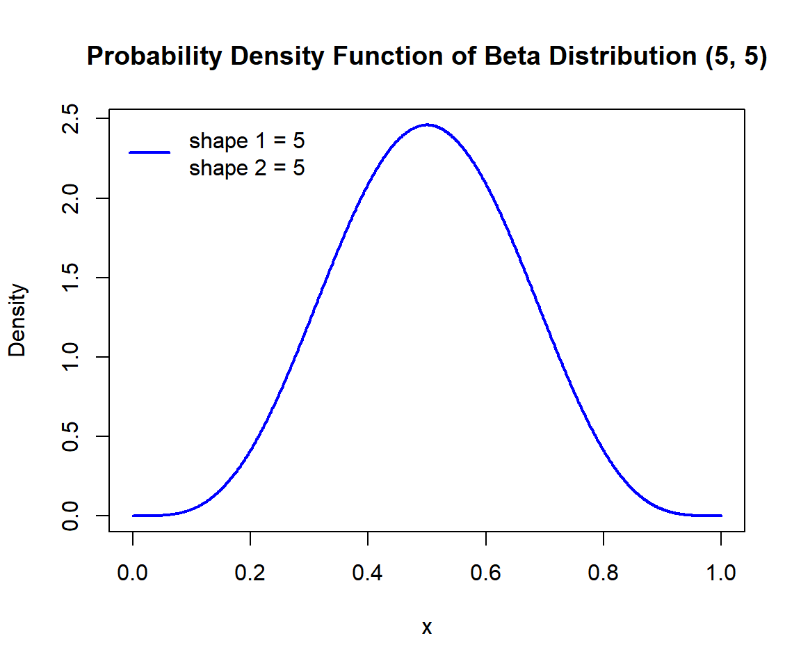

Probability Density Function (PDF) of a Beta Distribution in R

Multiple distributions:

Below is a plot of multiple beta distribution functions in one graph.

x1 = seq(0, 1, 1/1000); y1 = dbeta(x1, 2, 2)
x2 = seq(0, 1, 1/1000); y2 = dbeta(x2, 8, 2)
x3 = seq(0, 1, 1/1000); y3 = dbeta(x3, 2, 15)
x4 = seq(0.01, 0.99, 1/1000); y4 = dbeta(x4, 0.5, 0.5)
plot(x1, y1, type = "l",
     xlim = c(0, 1), ylim = range(c(y1, y2, y3, y4)),
     main = "Probability Density Functions of Beta Distributions",
     xlab = "x", ylab = "Density",
     lwd = 2, col = "blue")
points(x2, y2, type = "l", lwd = 2, col = "red")
points(x3, y3, type = "l", lwd = 2, col = "green")
points(x4, y4, type = "l", lwd = 2, col = "black")
# Add legend
legend("topright", c("shape1 = 2,    shape2 = 2",
                    "shape1 = 8,    shape2 = 2",
                    "shape1 = 2,    shape2 = 15",
                    "shape1 = 0.5, shape2 = 0.5"),
       lwd = c(2, 2, 2, 2),
       col = c("blue", "red", "green", "black"),
       bty = "n")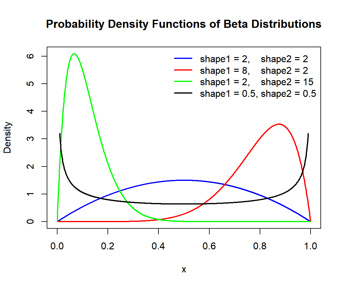

Probability Density Functions (PDFs) of Beta Distributions in R

3 Examples for Setting Parameters for Beta Distributions in R

To set the parameters for the beta distribution function, with \(\tt{shape\,1}=3\) and \(\tt{shape\,2}=4\).

For example, for qbeta(), the following are the same:

# The order of 3 and 4 matters here as the parameter names are not used.
# The first number 3 is shape1, and 4 is shape2.
qbeta(0.4, 3, 4)

[1] 0.3730797

# Or:
qbeta(0.4, shape1 = 3, shape2 = 4)

[1] 0.3730797

# Or:
qbeta(0.4, shape2 = 4, shape1 = 3)

[1] 0.3730797

4 rbeta(): Random Sampling from Beta Distributions in R

Sample 1000 observations from the beta distribution with \(\tt{shape\,1}=7\) and \(\tt{shape\,2}=15\):

rbeta(1000, 7, 15)

set.seed(123) # Line allows replication (use any number).
sample = rbeta(1000, 7, 15)
hist(sample,
     main = "Histogram of 1000 Observations from Beta Distribution
with Shape1 = 7 and Shape2 = 15",
     xlab = "x",
     col = "deepskyblue", border = "white")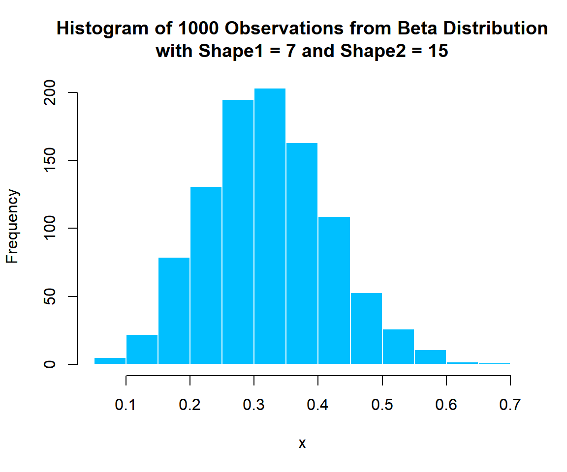

Histogram of Beta Distribution (7, 15) Random Sample in R

5 dbeta(): Probability Density Function for Beta Distributions in R

Calculate the density at \(x = 0.3\), in the beta distribution with \(\tt{shape\,1}=0.7\) and \(\tt{shape\,2}=0.4\):

dbeta(0.3, 0.7, 0.4)

[1] 0.5872993

x = seq(0.01, 0.99, 1/1000); y = dbeta(x, 0.7, 0.4)
plot(x, y, type = "l",
     xlim = c(0, 1), ylim = c(0,max(y)),
     main = "Probability Density Function of Beta Distribution
with Shape1 = 0.7 and Shape2 = 0.4",
     xlab = "x", ylab = "Density",
     lwd = 2, col = "blue")
# Add lines
segments(0.3, -1, 0.3, 0.5872993)
segments(-1, 0.5872993, 0.3, 0.5872993)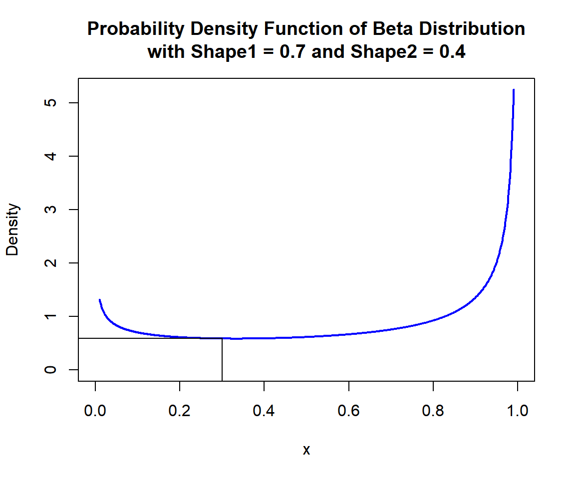

Probability Density Function (PDF) of Beta Distribution (0.7, 0.4) in R

6 pbeta(): Cumulative Distribution Function for Beta Distributions in R

Calculate the cumulative distribution at \(x = 0.45\), in the beta distribution with \(\tt{shape\,1}=6\) and \(\tt{shape\,2}=12\). That is, \(P(X \le 0.45)\):

pbeta(0.45, 6, 12)

[1] 0.8529322

x = seq(0, 1, 1/1000); y = pbeta(x, 6, 12)
plot(x, y, type = "l",
     xlim = c(0, 1), ylim = c(0,1),
     main = "Cumulative Distribution Function of Beta Distribution
with Shape1 = 6 and Shape2 = 12",
     xlab = "x", ylab = "Cumulative Distribution",
     lwd = 2, col = "blue")
# Add lines
segments(0.45, -1, 0.45, 0.8529322)
segments(-1, 0.8529322, 0.45, 0.8529322)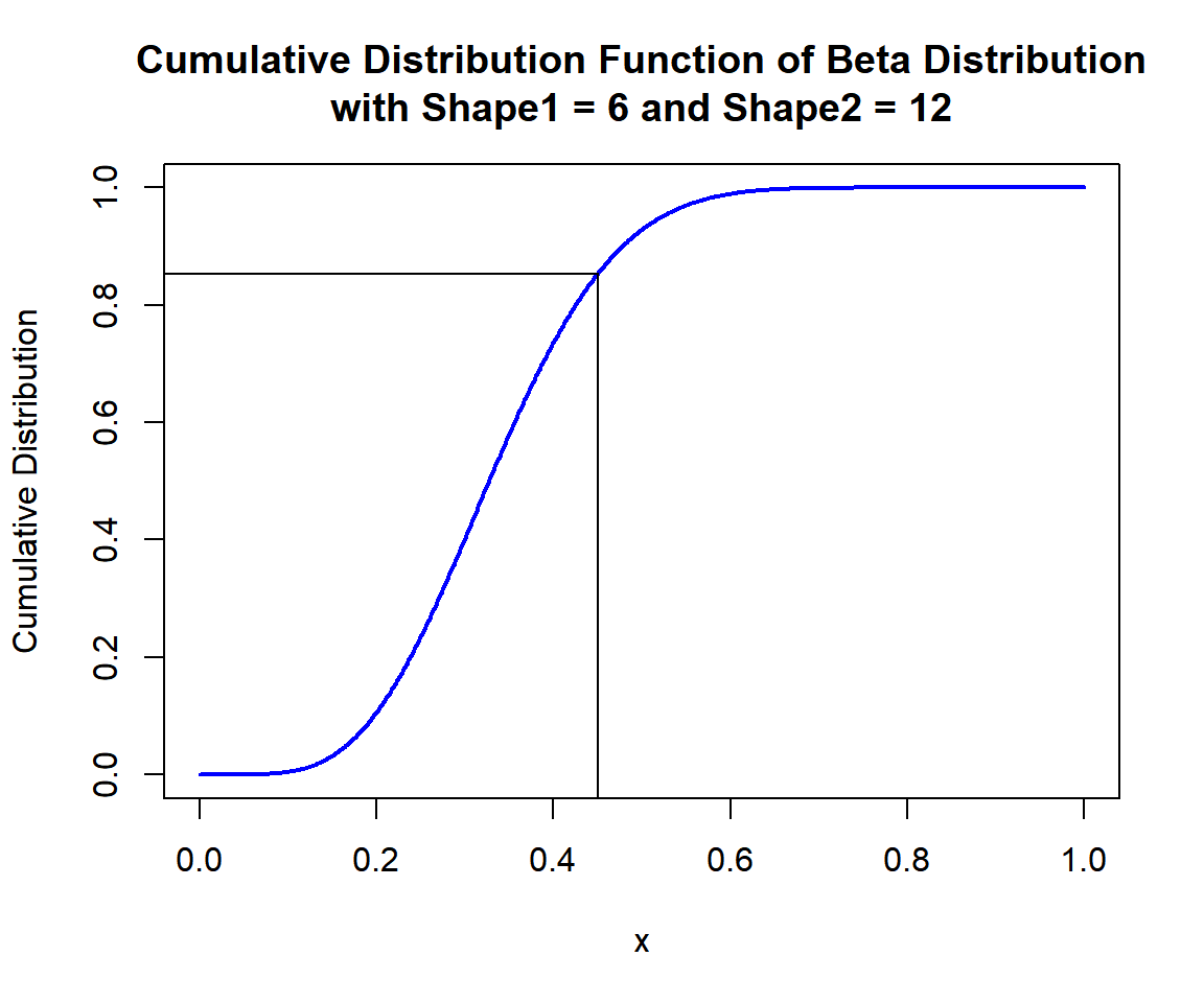

Cumulative Distribution Function (CDF) of Beta Distribution (6, 12) in R

x = seq(0, 1, 1/1000); y = dbeta(x, 6, 12)
plot(x, y, type = "l",
     xlim = c(0, 1), ylim = c(0, max(y)),
     main = "Probability Density Function of Beta Distribution
with Shape1 = 6 and Shape2 = 12",
     xlab = "x", ylab = "Density",
     lwd = 2, col = "blue")
# Add shaded region and legend
point = 0.45
polygon(x = c(x[x <= point], point),
        y = c(y[x <= point], 0),
        col = "limegreen")
legend("topright", c("Area = 0.8529322"),
       fill = c("limegreen"),
       inset = 0.01)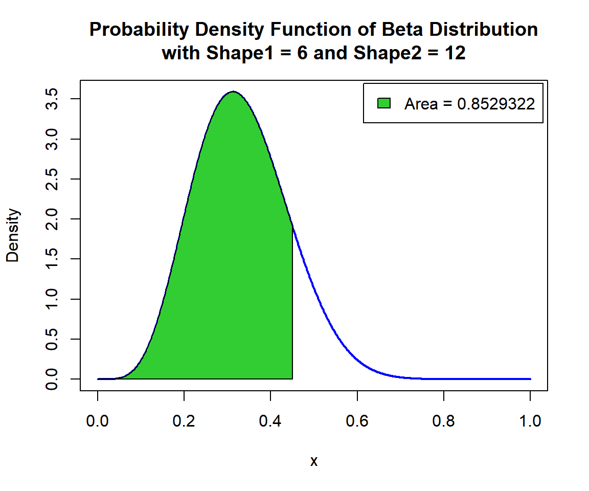

Shaded Probability Density Function (PDF) of Beta Distribution (6, 12) in R

For upper tail, at \(x = 0.45\), that is, \(P(X \ge 0.45) = 1 - P(X \le 0.45)\), set the "lower.tail" argument:

pbeta(0.45, 6, 12, lower.tail = FALSE)

[1] 0.1470678

x = seq(0, 1, 1/1000); y = dbeta(x, 6, 12)
plot(x, y, type = "l",
     xlim = c(0, 1), ylim = c(0, max(y)),
     main = "Shaded Upper Region: Probability Density Function of
Beta Distribution with Shape1 = 6 and Shape2 = 12",
     xlab = "x", ylab = "Density",
     lwd = 2, col = "blue")
# Add shaded region and legend
point = 0.45
polygon(x = c(point, x[x >= point]),
        y = c(0, y[x >= point]),
        col = "limegreen")
legend("topright", c("Area = 0.1470678"),
       fill = c("limegreen"),
       inset = 0.01)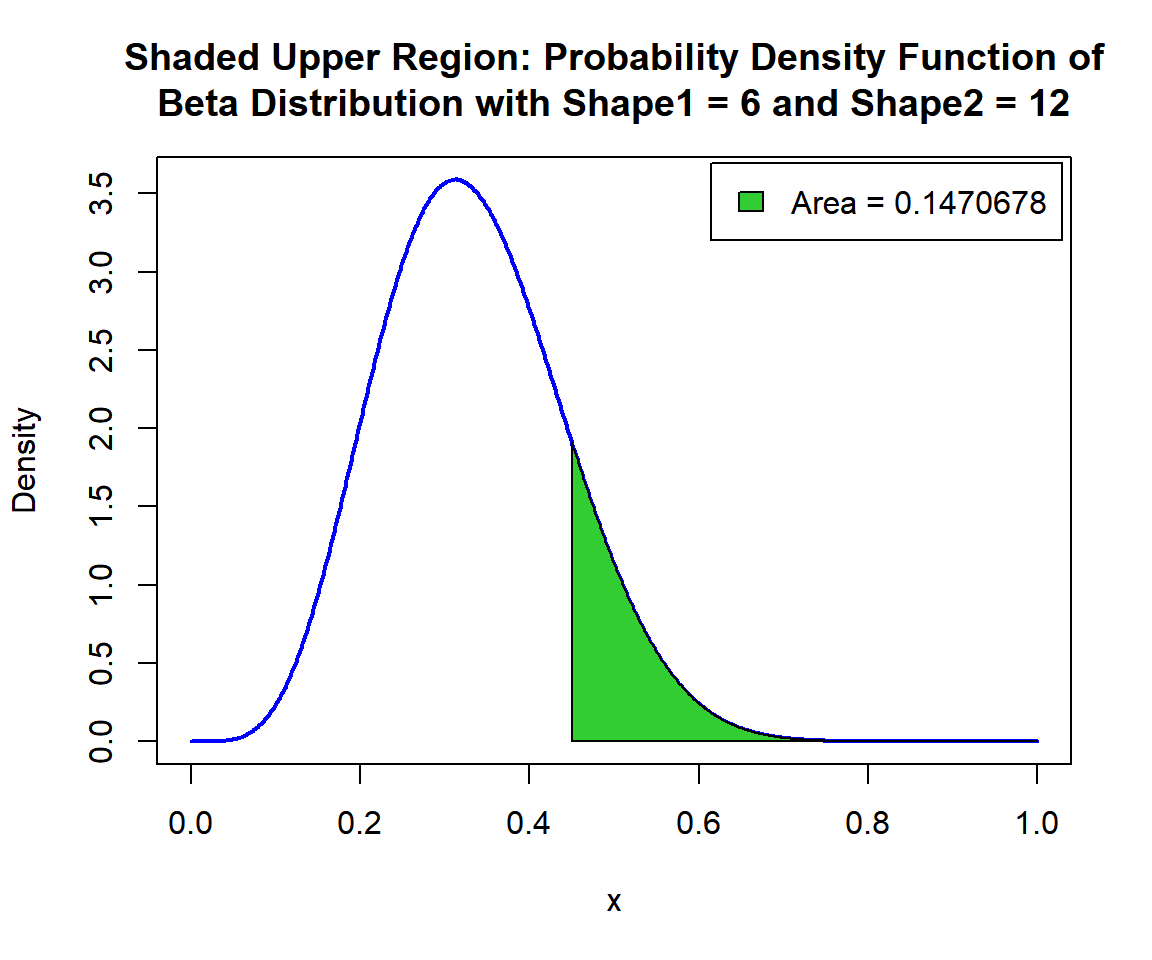

Shaded Upper Region: Probability Density Function (PDF) of Beta Distribution (6, 12) in R

7 qbeta(): Derive Quantile for Beta Distributions in R

Derive the quantile for \(p = 0.9\), in the beta distribution with \(\tt{shape\,1}=8.5\) and \(\tt{shape\,2}=7\). That is, \(x\) such that, \(P(X \le x)=0.9\):

qbeta(0.9, 8.5, 7)

[1] 0.7070644

x = seq(0, 1, 1/1000); y = pbeta(x, 8.5, 7)
plot(x, y, type = "l",
     xlim = c(0, 1), ylim = c(0,1),
     main = "Cumulative Distribution Function of Beta Distribution
with Shape1 = 8.5 and Shape2 = 7",
     xlab = "x", ylab = "Cumulative Distribution",
     lwd = 2, col = "blue")
# Add lines
segments(0.7070644, -1, 0.7070644, 0.9)
segments(-1, 0.9, 0.7070644, 0.9)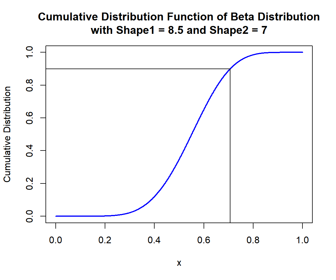

Cumulative Distribution Function (CDF) of Beta Distribution (8.5, 7) in R

x = seq(0, 1, 1/1000); y = dbeta(x, 8.5, 7)
plot(x, y, type = "l",
     xlim = c(0, 1), ylim = c(0, max(y)),
     main = "Probability Density Function of Beta Distribution
with Shape1 = 8.5 and Shape2 = 7",
     xlab = "x", ylab = "Density",
     lwd = 2, col = "blue")
# Add shaded region and legend
point = 0.7070644
polygon(x = c(x[x <= point], point),
        y = c(y[x <= point], 0),
        col = "limegreen")
legend("topright", c("Area = 0.9"),
       fill = c("limegreen"),
       inset = 0.01)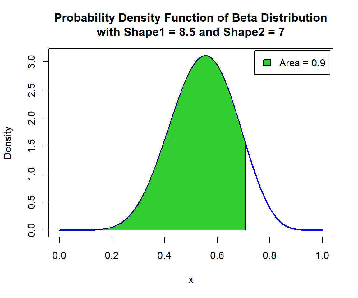

Shaded Probability Density Function (PDF) of Beta Distribution (8.5, 7) in R

For upper tail, for \(p = 0.1\), that is, \(x\) such that, \(P(X \ge x)=0.1\):

qbeta(0.1, 8.5, 7, lower.tail = FALSE)

[1] 0.7070644

x = seq(0, 1, 1/1000); y = dbeta(x, 8.5, 7)
plot(x, y, type = "l",
     xlim = c(0, 1), ylim = c(0, max(y)),
     main = "Shaded Upper Region: Probability Density Function of
Beta Distribution with Shape1 = 8.5 and Shape2 = 7",
     xlab = "x", ylab = "Density",
     lwd = 2, col = "blue")
# Add shaded region and legend
point = 0.7070644
polygon(x = c(point, x[x >= point]),
        y = c(0, y[x >= point]),
        col = "limegreen")
legend("topright", c("Area = 0.1"),
       fill = c("limegreen"),
       inset = 0.01)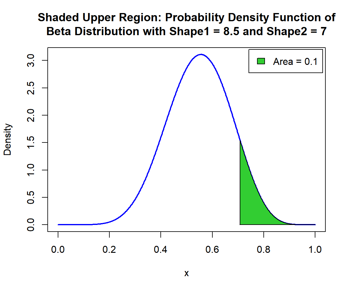

Shaded Upper Region: Probability Density Function (PDF) of Beta Distribution (8.5, 7) in R