Pooled Two Sample T-tests (Equal Variance) in R
- 1 Test Statistic for Pooled Two Sample T-test in R
- 2 Simple Pooled Two Sample T-test in R
- 3 Pooled Two Sample T-test Critical Value in R
- 4 Two-tailed Pooled Two Sample T-test in R
- 5 One-tailed Pooled Two Sample T-test in R
- 6 Pooled Two Sample T-test: Test Statistics, P-value & Degree of Freedom in R
- 7 Pooled Two Sample T-test: Estimates, Standard Error & Confidence Interval in R
Here, we discuss the pooled two sample t-test in R with interpretations, including, test statistics, p-values, critical values, confidence intervals, and standard errors.
The pooled two sample t-test in R can be performed with the
t.test() function from the base "stats" package.
The pooled two sample t-test is also the independent (unpaired) two sample t-test with equal variance assumption. When the population variances are assumed to be equal, it can be used to test whether the difference between the means of the two populations where two independent random samples come from is equal to a certain value (which is stated in the null hypothesis) or not.
In the pooled two sample t-test, the test statistic follows a Student’s t-distribution when the null hypothesis is true.
| Question | Are the means equal, or difference equal to \(\mu_0\)? | Is mean x greater than mean y, or difference greater than \(\mu_0\)? | Is mean x less than mean y, or difference less than \(\mu_0\)? |
| Form of Test | Two-tailed, with \(\sigma^2_x = \sigma^2_y\) assumption | Right-tailed test, with \(\sigma^2_x = \sigma^2_y\) assumption | Left-tailed test, with \(\sigma^2_x = \sigma^2_y\) assumption |
| Null Hypothesis, \(H_0\) | \(\mu_x = \mu_y;\) \(\quad\) \(\mu_x - \mu_y = \mu_0\) | \(\mu_x = \mu_y;\) \(\quad\) \(\mu_x-\mu_y = \mu_0\) | \(\mu_x = \mu_y;\) \(\quad\) \(\mu_x-\mu_y = \mu_0\) |
| Alternate Hypothesis, \(H_1\) | \(\mu_x \neq \mu_y;\) \(\quad\) \(\mu_x-\mu_y \neq \mu_0\) | \(\mu_x > \mu_y;\) \(\quad\) \(\mu_x-\mu_y > \mu_0\) | \(\mu_x < \mu_y;\) \(\quad\) \(\mu_x-\mu_y < \mu_0\) |
Sample Steps to Run a Pooled Two Sample T-test:
# Create the data samples for the pooled two sample t-test

data_x = c(14.1, 13.2, 16.7, 11.3,
           9.5, 12.7, 13.5, 8.9)
data_y = c(16.4, 14.7, 6.8, 17.4, 7.2)

# Run the pooled two sample t-test with specifications

t.test(data_x, data_y, var.equal = TRUE,
       alternative = "less",
       mu = 0, conf.level = 0.95)
    Two Sample t-test

data:  data_x and data_y
t = -0.0059423, df = 11, p-value = 0.4977
alternative hypothesis: true difference in means is less than 0
95 percent confidence interval:
    -Inf 3.76526
sample estimates:
mean of x mean of y
12.4875 12.5000 | Argument | Usage |
| x, y | The two sample data values |
| x ~ y | x contains the two sample data values, y specifies the group they belong |
| var.equal | Set to TRUE for pooled two sample t-test (default =
FALSE) |
| alternative | Set alternate hypothesis as "greater", "less", or the default "two.sided" |
| mu | The difference between the population mean values in null hypothesis |
| conf.level | Level of confidence for the test and confidence interval (default = 0.95) |
Creating a Pooled Two Sample T-test Object:
# Create data
data_x = rnorm(40); data_y = rnorm(60)

# Create object
test_object = t.test(data_x, data_y,
                     var.equal = TRUE,
                     alternative = "two.sided",
                     mu = 0, conf.level = 0.95)

# Extract a component
test_object$statistic
t
-0.4027924 | Test Component | Usage |
| test_object$statistic | t-statistic value |
| test_object$p.value | P-value |
| test_object$parameter | Degrees of freedom |
| test_object$estimate | Point estimates or sample means |
| test_object$stderr | Standard error value |
| test_object$conf.int | Confidence interval |
1 Test Statistic for Pooled Two Sample T-test in R
The pooled two sample t-test given its independent samples and equal variance assumption has test statistics, \(t\), of the form:
\[t = \frac{(\bar x - \bar y) - \mu_0}{s_p \cdot \sqrt{\frac{1}{n_x}+\frac{1}{n_y}}},\]
where \[s_p = \sqrt{\frac{\left(n_x-1\right)s_{x}^2+\left(n_y-1\right)s_{y}^2}{n_x+n_y-2}}.\]
For independent random samples that come from normal distributions or for large sample sizes (for example, \(n_x > 30\) and \(n_y > 30\)), \(t\) is said to follow the Student’s t-distribution when the null hypothesis and the equal variances assumption are true, with the degrees of freedom as \(n_x+n_y-2\).
\(\bar x\) and \(\bar y\) are the sample means,
\(\mu_0\) is the difference between the population mean values to be tested and set in the null hypothesis,
\(s_x\) and \(s_y\) are the sample standard deviations,
\(s_x^2\) and \(s_y^2\) are the sample variances,
\(s_p^2\) is the pooled sample variance, and
\(n_x\) and \(n_y\) are the sample sizes.
See also one sample t-tests and two sample t-tests (independent & unequal variance and dependent or paired samples).
For a non-parametric test, see the Wilcoxon rank-sum test.
2 Simple Pooled Two Sample T-test in R
Enter the data by hand.
data_x = c(53.4, 53.5, 49.1, 55.1, 53.1,
          44.6, 37.5, 38.1, 53.7, 49.4)
data_y = c(48.0, 48.1, 49.7, 56.7, 50.7,
          43.3, 52.2, 47.1, 44.0, 50.6,
          42.9, 52.3, 52.4, 52.5, 50.8)
For data_x as the \(x\) group and data_y as the \(y\) group.
For the following null hypothesis \(H_0\), and alternative hypothesis \(H_1\), with the level of significance \(\alpha=0.05\).
\(H_0:\) the difference between the population means is equal to 0 (\(\mu_x - \mu_y = 0\)).
\(H_1:\) the difference between the population means is not equal to 0 (\(\mu_x - \mu_y \neq 0\), hence the default two-sided).
Because the level of significance is \(\alpha=0.05\), the level of confidence is \(1 - \alpha = 0.95\).
The t.test() function has the default
alternative as "two.sided", the default difference
between the means as 0, and the default level of
confidence as 0.95, hence, you do not need to specify the
"alternative", "mu", and "conf.level" arguments in this
case.
Or:
    Two Sample t-test

data:  data_x and data_y
t = -0.32224, df = 23, p-value = 0.7502
alternative hypothesis: true difference in means is not equal to 0
95 percent confidence interval:
 -4.971099  3.631099
sample estimates:
mean of x mean of y
    48.75     49.42
The first sample mean, \(\bar x\), is 48.75, and the second sample mean, \(\bar y\), is 49.42,
test statistic, \(t\), is -0.32224,
the degrees of freedom, \(n_x+n_y-2\), is 23,
the p-value, \(p\), is 0.7502,
the 95% confidence interval is [-4.971099, 3.631099].
Interpretation:
P-value: With the p-value (\(p = 0.7502\)) being greater than the level of significance 0.05, we fail to reject the null hypothesis that the difference between the population means is equal to 0.
\(t\)-statistic: With test statistics value (\(t = -0.32224\)) being between the two critical values, \(-t_{n_x+n_y-2,\alpha/2}=\text{qt(0.025, 23)}=-2.0686576\) and \(t_{n_x+n_y-2,\alpha/2}=\text{qt(0.975, 23)}=2.0686576\) (or not in the shaded region), we fail to reject the null hypothesis that the difference between the population means is equal to 0.
Confidence Interval: With the null hypothesis difference between the means value (\(\mu_x - \mu_y = 0\)) being inside the confidence interval, \([-4.971099, 3.631099]\), we fail to reject the null hypothesis that the difference between the population means is equal to 0.
x = seq(-4, 4, 1/1000); y = dt(x, df=23)
plot(x, y, type = "l",
     xlim = c(-4, 4), ylim = c(-0.03, max(y)),
     main = "Pooled Two Sample Student's T-test
Shaded Region for Simple T-test",
     xlab = "x", ylab = "Density",
     lwd = 2, col = "blue")
abline(h=0)
# Add shaded region and legend
point1 = qt(0.025, 23); point2 = qt(0.975, 23)
polygon(x = c(-4, x[x <= point1], point1),
        y = c(0, y[x <= point1], 0),
        col = "blue")
polygon(x = c(x[x >= point2], 4, point2),
        y = c(y[x >= point2], 0, 0),
        col = "blue")
legend("topright", c("Area = 0.05"),
       fill = c("blue"), inset = 0.01)
# Add critical value and t-value
arrows(0, 0.1, -0.32224, 0)
text(0, 0.12, "t = -0.32224")
text(-2.068658, -0.02, expression(-t[df][','][alpha/2]==-2.068658))
text(2.068658, -0.02, expression(t[df][','][alpha/2]==2.068658))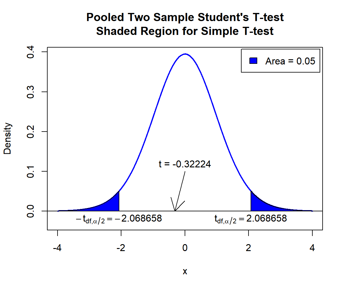
Pooled Two Sample Student’s T-test Shaded Region for Simple T-test in R
See line charts, shading areas under a curve, lines & arrows on plots, mathematical expressions on plots, and legends on plots for more details on making the plot above.
3 Pooled Two Sample T-test Critical Value in R
To get the critical value for a pooled two sample t-test in R, you
can use the qt() function for Student’s t-distribution to
derive the quantile associated with the given level of significance
value \(\alpha\).
For two-tailed test with level of significance \(\alpha\). The critical values are: qt(\(\alpha/2\), df) and qt(\(1-\alpha/2\), df).
For one-tailed test with level of significance \(\alpha\). The critical value is: for left-tailed, qt(\(\alpha\), df); and for right-tailed, qt(\(1-\alpha\), df).
Example:
For \(\alpha = 0.1\), and \(\text{df = 28}\).
Two-tailed:
[1] -1.701131[1] 1.701131One-tailed:
[1] -1.312527[1] 1.3125274 Two-tailed Pooled Two Sample T-test in R
Using the CO2 data from the "datasets" package with 10 sample rows from 84 rows below:
   Plant        Type  Treatment conc uptake
1    Qn1      Quebec nonchilled   95   16.0
15   Qn3      Quebec nonchilled   95   16.2
16   Qn3      Quebec nonchilled  175   32.4
31   Qc2      Quebec    chilled  250   35.0
37   Qc3      Quebec    chilled  175   21.0
51   Mn2 Mississippi nonchilled  175   22.0
54   Mn2 Mississippi nonchilled  500   32.4
70   Mc1 Mississippi    chilled 1000   21.9
80   Mc3 Mississippi    chilled  250   17.9
84   Mc3 Mississippi    chilled 1000   19.9
For "Quebec" as the \(x\) group versus "Mississippi" as the \(y\) group.
For the following null hypothesis \(H_0\), and alternative hypothesis \(H_1\), with the level of significance \(\alpha=0.1\).
\(H_0:\) population mean of group \(x\) minus population mean of group \(y\) is equal to 18 (\(\mu_x - \mu_y = 18\)).
\(H_1:\) population mean of group \(x\) minus population mean of group \(y\) is not equal to 18 (\(\mu_x - \mu_y \neq 18\), hence the default two-sided).
Because the level of significance is \(\alpha=0.1\), the level of confidence is \(1 - \alpha = 0.9\).
# This example uses t.test(x ~ y). For t.test(x, y), see other examples above or below.
t.test(uptake ~ Type, data = CO2, var.equal = TRUE,
       alternative = "two.sided",
       mu = 18, conf.level = 0.9)
    Two Sample t-test

data:  uptake by Type
t = -2.7829, df = 82, p-value = 0.006685
alternative hypothesis: true difference in means between group Quebec and group Mississippi is not equal to 18
90 percent confidence interval:
  9.466963 15.852085
sample estimates:
     mean in group Quebec mean in group Mississippi
                 33.54286                  20.88333
Interpretation:
P-value: With the p-value (\(p = 0.006685\)) being lower than the level of significance 0.1, we reject the null hypothesis that the difference between the population means is equal to 18.
\(t\)-statistic: With test statistics value (\(t = -2.7829\)) being inside the critical region (shaded area), that is, \(t = -2.7829\) less than \(-t_{n_x+n_y-2,\alpha/2}=\text{qt(0.05, 82)}=-1.6636492\), we reject the null hypothesis that the difference between the population means is equal to 18.
Confidence Interval: With the null hypothesis difference between the means value (\(\mu_x - \mu_y = 18\)) being outside the confidence interval, \([9.466963, 15.852085]\), we reject the null hypothesis that the difference between the population means is equal to 18.
x = seq(-4, 4, 1/1000); y = dt(x, df=82)
plot(x, y, type = "l",
     xlim = c(-4, 4), ylim = c(-0.03, max(y)),
     main = "Pooled Two Sample Student's T-test
Shaded Region for Two-tailed Test",
     xlab = "x", ylab = "Density",
     lwd = 2, col = "blue")
abline(h=0)
# Add shaded region and legend
point1 = qt(0.05, 82); point2 = qt(0.95, 82)
polygon(x = c(-4, x[x <= point1], point1),
        y = c(0, y[x <= point1], 0),
        col = "blue")
polygon(x = c(x[x >= point2], 4, point2),
        y = c(y[x >= point2], 0, 0),
        col = "blue")
legend("topright", c("Area = 0.1"),
       fill = c("blue"), inset = 0.01)
# Add critical value and t-value
arrows(-2.7829, 0.25, -2.7829, 0)
text(-2.7829, 0.27, expression(t==-2.7829))
text(-1.663649, -0.02, expression(-t[df][','][alpha/2]==-1.663649))
text(1.663649, -0.02, expression(t[df][','][alpha/2]==1.663649))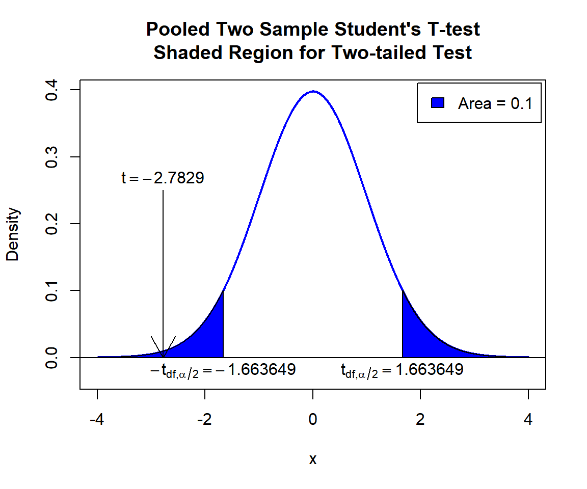
Pooled Two Sample Student’s T-test Shaded Region for Two-tailed Test in R
5 One-tailed Pooled Two Sample T-test in R
Right Tailed Test
Using the attitude data from the "datasets" package with 10 sample rows from 30 rows below:
   rating complaints privileges learning raises critical advance
1      43         51         30       39     61       92      45
3      71         70         68       69     76       86      48
6      43         55         49       44     54       49      34
15     77         77         54       72     79       77      46
17     74         85         64       69     79       79      63
24     40         37         42       58     50       57      49
26     66         77         66       63     88       76      72
27     78         75         58       74     80       78      49
29     85         85         71       71     77       74      55
30     82         82         39       59     64       78      39
For "learning" as the \(x\) group versus "privileges" as the \(y\) group.
For the following null hypothesis \(H_0\), and alternative hypothesis \(H_1\), with the level of significance \(\alpha=0.1\).
\(H_0:\) population mean of group \(x\) and population mean of group \(y\) are equal (\(\mu_x - \mu_y = 0\)).
\(H_1:\) population mean of group \(x\) is greater than population mean of group \(y\) (\(\mu_x - \mu_y > 0\), hence one-sided).
Because the level of significance is \(\alpha=0.1\), the level of confidence is \(1 - \alpha = 0.9\).
t.test(attitude$learning, attitude$privileges,
       var.equal = TRUE,
       alternative = "greater",
       mu = 0, conf.level = 0.9)
    Two Sample t-test

data:  attitude$learning and attitude$privileges
t = 1.0445, df = 58, p-value = 0.1503
alternative hypothesis: true difference in means is greater than 0
90 percent confidence interval:
 -0.7794191        Inf
sample estimates:
mean of x mean of y
 56.36667  53.13333
Interpretation:
P-value: With the p-value (\(p = 0.1503\)) being greater than the level of significance 0.1, we fail to reject the null hypothesis that the difference between the population means is equal to 0.
\(t\)-statistic: With test statistics value (\(t = 1.0445\)) being outside the critical region (shaded area), that is, \(t = 1.0445\) less than \(t_{n_x+n_y-2,\alpha}=\text{qt(0.9, 58)}=1.2963189\), we fail to reject the null hypothesis that the difference between the population means is equal to 0.
Confidence Interval: With the null hypothesis difference between the means value (\(\mu_x - \mu_y = 0\)) being inside the confidence interval, \([-0.7794191, \infty)\), we fail to reject the null hypothesis that the difference between the population means is equal to 0.
x = seq(-4, 4, 1/1000); y = dt(x, df=58)
plot(x, y, type = "l",
     xlim = c(-4, 4), ylim = c(-0.03, max(y)),
     main = "Pooled Two Sample Student's T-test
Shaded Region for Right-tailed Test",
     xlab = "x", ylab = "Density",
     lwd = 2, col = "blue")
abline(h=0)
# Add shaded region and legend
point = qt(0.9, 58)
polygon(x = c(x[x >= point], 4, point),
        y = c(y[x >= point], 0, 0),
        col = "blue")
legend("topright", c("Area = 0.1"),
       fill = c("blue"), inset = 0.01)
# Add critical value and t-value
arrows(0, 0.1, 1.0445, 0)
text(0, 0.12, expression(t==1.0445))
text(1.296319, -0.02, expression(t[df][','][alpha]==1.296319))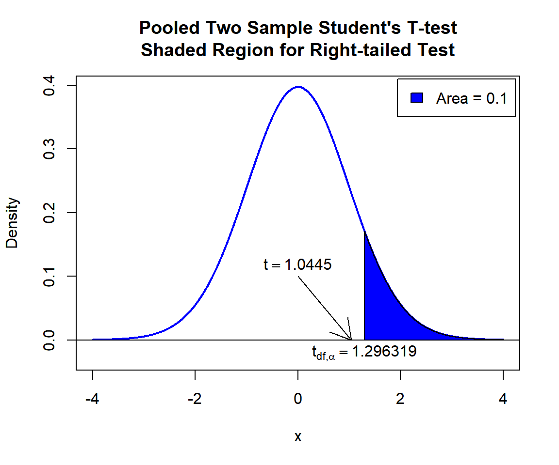
Pooled Two Sample Student’s T-test Shaded Region for Right-tailed Test in R
Left Tailed Test
For "critical" as the \(x\) group versus "raises" as the \(y\) group.
For the following null hypothesis \(H_0\), and alternative hypothesis \(H_1\), with the level of significance \(\alpha=0.2\).
\(H_0:\) population mean of group \(x\) minus population mean of group \(y\) is equal to 15 (\(\mu_x - \mu_y = 15\)).
\(H_1:\) population mean of group \(x\) minus population mean of group \(y\) is less than 15 (\(\mu_x - \mu_y < 15\), hence one-sided).
Because the level of significance is \(\alpha=0.2\), the level of confidence is \(1 - \alpha = 0.8\).
t.test(attitude$critical, attitude$raises,
       var.equal = TRUE,
       alternative = "less",
       mu = 15, conf.level = 0.8)
    Two Sample t-test

data:  attitude$critical and attitude$raises
t = -1.8571, df = 58, p-value = 0.03419
alternative hypothesis: true difference in means is less than 15
80 percent confidence interval:
     -Inf 12.35516
sample estimates:
mean of x mean of y
 74.76667  64.63333
Interpretation:
P-value: With the p-value (\(p = 0.03419\)) being less than the level of significance 0.2, we reject the null hypothesis that the difference between the population means is equal to 15.
\(t\)-statistic: With test statistics value (\(t = -1.8571\)) being inside the critical region (shaded area), that is, \(t = -1.8571\) less than \(-t_{n_x+n_y-2,\alpha}=\text{qt(0.2, 58)}=-0.8478625\), we reject the null hypothesis that the difference between the population means is equal to 15.
Confidence Interval: With the null hypothesis difference between the means value (\(\mu_x - \mu_y = 15\)) being outside the confidence interval, \((-\infty, 12.35516]\), we reject the null hypothesis that the difference between the population means is equal to 15.
x = seq(-4, 4, 1/1000); y = dt(x, df=58)
plot(x, y, type = "l",
     xlim = c(-4, 4), ylim = c(-0.03, max(y)),
     main = "Pooled Two Sample Student's T-test
Shaded Region for Left-tailed Test",
     xlab = "x", ylab = "Density",
     lwd = 2, col = "blue")
abline(h=0)
# Add shaded region and legend
point = qt(0.2, 58)
polygon(x = c(-4, x[x <= point], point),
        y = c(0, y[x <= point], 0),
        col = "blue")
legend("topright", c("Area = 0.2"),
       fill = c("blue"), inset = 0.01)
# Add critical value and t-value
arrows(-1.8571, 0.25, -1.8571, 0)
text(-1.8571, 0.27, expression(t==-1.8571))
text(-0.8478625, -0.02, expression(-t[df][','][alpha]==-0.8478625))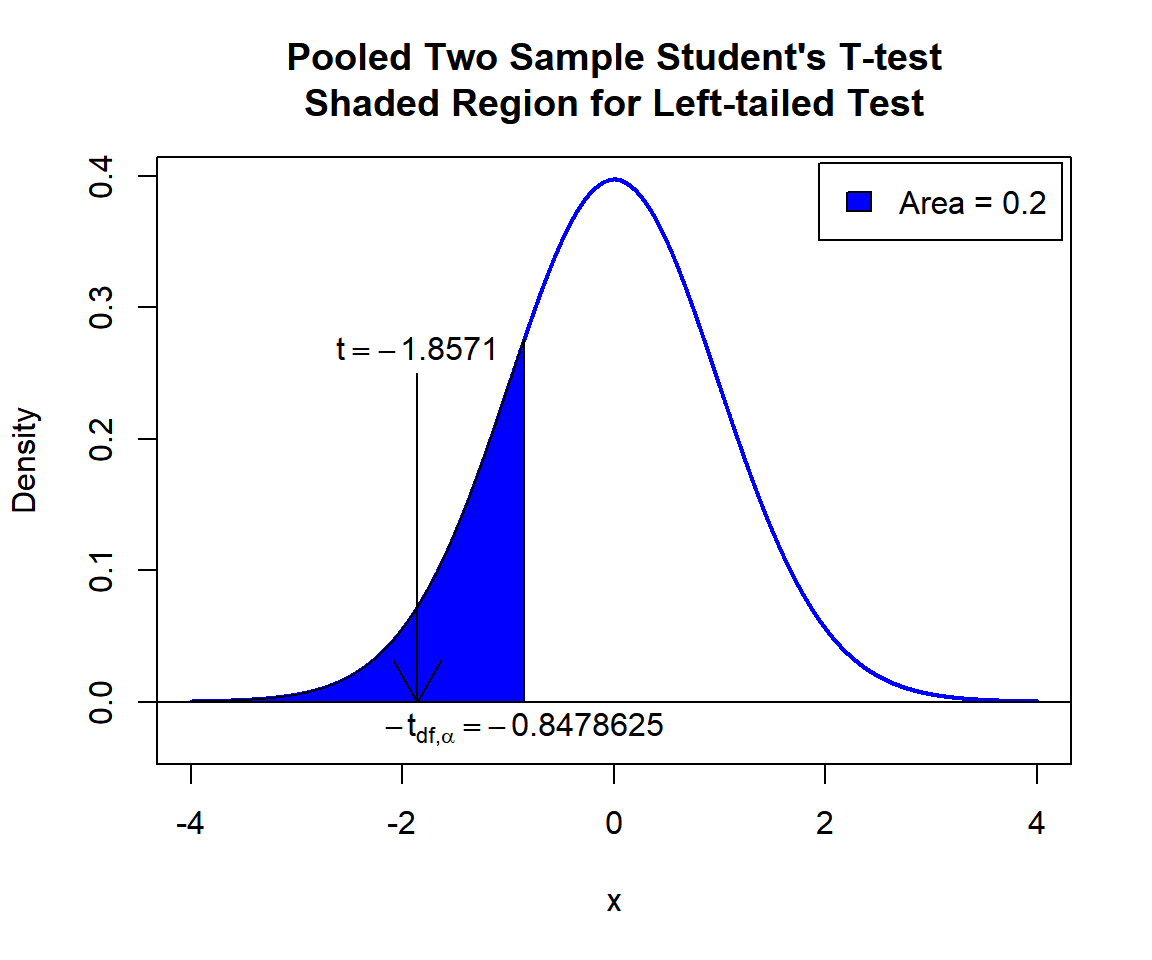
Pooled Two Sample Student’s T-test Shaded Region for Left-tailed Test in R
6 Pooled Two Sample T-test: Test Statistics, P-value & Degree of Freedom in R
Here for a pooled two sample t-test, we show how to get the test
statistics (or t-value), p-values, and degrees of freedom from the
t.test() function in R, or by written code.
data_x = attitude$raises; data_y = attitude$learning
test_object = t.test(data_x, data_y, var.equal = TRUE,
                     alternative = "two.sided",
                     mu = 0, conf.level = 0.9)
test_object
    Two Sample t-test

data:  data_x and data_y
t = 2.8877, df = 58, p-value = 0.005446
alternative hypothesis: true difference in means is not equal to 0
90 percent confidence interval:
  3.481432 13.051901
sample estimates:
mean of x mean of y
 64.63333  56.36667
To get the test statistic or t-value:
\[t = \frac{(\bar x - \bar y) - \mu_0}{s_p \cdot \sqrt{\frac{1}{n_x}+\frac{1}{n_y}}},\] where \[s_p = \sqrt{\frac{\left(n_x-1\right)s_{x}^2+\left(n_y-1\right)s_{y}^2}{n_x+n_y-2}}.\]
       t
2.887668 [1] 2.887668Same as:
mu = 0; df = length(data_x) + length(data_y) - 2
sp = sqrt(((length(data_x)-1)*var(data_x) + (length(data_y)-1)*var(data_y))/df)
(mean(data_x)-mean(data_y)-mu)/(sp*sqrt((1/length(data_x))+(1/length(data_y))))
[1] 2.887668To get the p-value:
Two-tailed: For positive test statistic (\(t^+\)), and negative test statistic (\(t^-\)).
\(Pvalue = 2*P(t_{n_x+n_y-2}>t^+)\) or \(Pvalue = 2*P(t_{n_x+n_y-2}<t^-)\).
One-tailed: For right-tail, \(Pvalue = P(t_{n_x+n_y-2}>t)\) or for left-tail, \(Pvalue = P(t_{n_x+n_y-2}<t)\).
[1] 0.005446193Same as:
Note that the p-value depends on the \(\text{test statistics}\) (2.887668) and
\(\text{degrees of freedom}\) (58). We
also use the distribution function pt() for the Student’s
t-distribution in R.
[1] 0.005446198[1] 0.005446198One-tailed example:
To get the degrees of freedom:
The degrees of freedom are \(n_x + n_y - 2\).
df
58 [1] 58Same as:
[1] 587 Pooled Two Sample T-test: Estimates, Standard Error & Confidence Interval in R
Here for a pooled two sample t-test, we show how to get the sample
means, standard error estimate, and confidence interval from the
t.test() function in R, or by written code.
data_x = attitude$privileges; data_y = attitude$advance
test_object = t.test(data_x, data_y, var.equal = TRUE,
                     alternative = "two.sided",
                     mu = 0, conf.level = 0.95)
test_object
    Two Sample t-test

data:  data_x and data_y
t = 3.4947, df = 58, p-value = 0.0009162
alternative hypothesis: true difference in means is not equal to 0
95 percent confidence interval:
  4.357599 16.042401
sample estimates:
mean of x mean of y
 53.13333  42.93333
To get the point estimates or sample means:
\[\bar x = \frac{1}{n}\sum_{i=1}^{n} x_i \;, \quad \bar y = \frac{1}{n}\sum_{i=1}^{n} y_i.\]
mean of x mean of y
53.13333 42.93333 [1] 53.13333 42.93333Same as:
[1] 53.13333[1] 42.93333To get the standard error estimate:
\[\widehat {SE} = s_p \cdot \sqrt{\frac{1}{n_x}+\frac{1}{n_y}} \quad ,\]
where \[s_p = \sqrt{\frac{\left(n_x-1\right)s_{x}^2+\left(n_y-1\right)s_{y}^2}{n_x+n_y-2}}.\]
[1] 2.918694Same as:
df = length(data_x) + length(data_y) - 2
sp = sqrt(((length(data_x)-1)*var(data_x) + (length(data_y)-1)*var(data_y))/df)
sp*sqrt((1/length(data_x))+(1/length(data_y)))
[1] 2.918694To get the confidence interval for \(\mu_x - \mu_y\):
For two-tailed: \[CI = \left[(\bar x-\bar y) - t_{n_x+n_y-2,\alpha/2}*\widehat {SE} \;,\; (\bar x-\bar y) + t_{n_x+n_y-2,\alpha/2}*\widehat {SE} \right].\]
For right one-tailed: \[CI = \left[(\bar x-\bar y) - t_{n_x+n_y-2,\alpha}*\widehat {SE} \;,\; \infty \right).\]
For left one-tailed: \[CI = \left(-\infty \;,\; (\bar x-\bar y) + t_{n_x+n_y-2,\alpha}*\widehat {SE} \right].\]
[1]  4.357599 16.042401
attr(,"conf.level")
[1] 0.95[1] 4.357599 16.042401Same as:
Note that the critical values depend on the \(\alpha\) (0.05) and \(\text{degrees of freedom}\) (58).
alpha = 0.05
df = length(data_x) + length(data_y) - 2
sp = sqrt(((length(data_x)-1)*sd(data_x)^2 + (length(data_y)-1)*sd(data_y)^2)/df)
SE = sp*sqrt((1/length(data_x))+(1/length(data_y)))
l = (mean(data_x) - mean(data_y)) - qt(1-alpha/2, df)*SE
u = (mean(data_x) - mean(data_y)) + qt(1-alpha/2, df)*SE
c(l, u)
[1] 4.357599 16.042401One-tailed example:
The feedback form is a Google form but it does not collect any personal information.
Please click on the link below to go to the Google form.
Thank You!
Go to Feedback Form
Copyright © 2020 - 2026. All Rights Reserved by Stats Codes