Spearman’s Rank Correlation Coefficient Tests in R
- 1 Test Statistic for Spearman’s Rank Correlation Coefficient Test in R
- 2 Simple Spearman’s Rank Correlation Coefficient Test in R
- 3 Two-tailed Spearman’s Rank Correlation Coefficient Test in R
- 4 One-tailed Spearman’s Rank Correlation Coefficient Test in R
- 5 Spearman’s Rank Correlation Coefficient Test: Estimate, Test Statistics & P-value in R
Here, we discuss the Spearman’s rank correlation coefficient test in R with interpretations, including, rank correlation, test statistics, and p-values.
The Spearman’s rank correlation coefficient test in R can be
performed with the cor.test() function from the base
"stats" package.
The Spearman’s rank correlation coefficient test can be used to test whether there is a rank correlation between two variables or if there is none as stated in the null hypothesis. It is a non-parametric alternative to the Pearson’s correlation coefficient test.
In the Spearman’s rank correlation coefficient test, the test statistic is based on the correlation between the ranks of the observed values within each sample, and it follows a Student’s t-distribution when the null hypothesis is true.
| Question | Is there a rank correlation between x and y? | Is there a positive rank correlation between x and y? | Is there a negative rank correlation between x and y? |
| Form of Test | Two-tailed | Right-tailed test | Left-tailed test |
| Null Hypothesis, \(H_0\) | \(\rho_s = 0\) | \(\rho_s = 0\) | \(\rho_s = 0\) |
| Alternate Hypothesis, \(H_1\) | \(\rho_s \neq 0\) | \(\rho_s > 0\) | \(\rho_s < 0\) |
Sample Steps to Run a Spearman’s Rank Correlation Coefficient Test:
# Create the data samples for the Spearman's rank correlation coefficient test
# Values are paired based on matching position in each sample

data_x = c(3.4, 2.5, 2.7, 2.0, 1.9)
data_y = c(6.8, 7.3, 8.1, 7.4, 6.7)

# Run the Spearman's rank correlation coefficient test with specifications

cor.test(data_x, data_y,
         alternative = "two.sided",
         method = "spearman")
    Spearman's rank correlation rho

data:  data_x and data_y
S = 14, p-value = 0.6833
alternative hypothesis: true rho is not equal to 0
sample estimates:
rho
0.3 | Argument | Usage |
| x, y | The two sample data values |
| alternative | Set alternate hypothesis as "greater", "less", or the default "two.sided" |
| method | Set to "spearman", the default is "pearson" |
| exact | For n<=1290 and no rank ties: set to FALSE to
compute p-value based on t-distribution, (default =
TRUE) |
| continuity | Set to TRUE for continuity correction for non-exact
p-value |
Creating a Spearman’s Rank Correlation Coefficient Test Object:
# Create data
data_x = rnorm(60); data_y = rnorm(60)

# Create object
cor_object = cor.test(data_x, data_y,
                      alternative = "two.sided",
                      method = "spearman", conf.level = 0.95)

# Extract a component
cor_object$statistic
S
32518 | Test Component | Usage |
| cor_object$statistic | Test-statistic value |
| cor_object$p.value | P-value |
| cor_object$estimate | Sample rank correlation coefficient |
1 Test Statistic for Spearman’s Rank Correlation Coefficient Test in R
With \(\text{rank}(4, 6, 6, 8, 10, 10, 10) = (1, 2.5, 2.5, 4, 6, 6, 6)\).
Let \(r(x_i)\), be the rank for \(x_i\) among the \(x\) sample data values,
\(r(y_i)\), be the rank for \(y_i\) among the \(y\) sample data values,
\(\bar r(x)\) and \(\bar r(y)\) are the mean ranks for \(x\) and \(y\),
\(n \in \{3, 4, 5 ...\}\) is the number of sample pairs.
Similar to Pearson’s correlation coefficient, the sample Spearman’s rank correlation coefficient is:
\[ r_s = \frac{\sum ^n _{i=1}[r(x_i) - \bar r(x)][r(y_i) - \bar r(y)]}{\sqrt{\sum ^n _{i=1}[r(x_i) - \bar r(x)]^2} \sqrt{\sum ^n _{i=1}[r(y_i) - \bar r(y)]^2}}\]
If all the ranks are unique with no ties, then \(r_s\) can be calculated as:
\[ r_s = 1 - \frac{6 \sum ^n _{i=1} d_i^2}{n(n^2-1)},\] where \(d_i = r(x_i) - r(y_i)\) for each \(i\).
Large Samples:
In R, for large sample pairs (\(n>1290\)) or cases with rank ties, the test has test statistics, \(t\), of the form:
\[t = \frac{r_s}{\sqrt{\frac{1 - r_s^2}{n-2}}}.\]
\(t\) follows the Student’s t-distribution with \(n-2\) degrees of freedom (\(t_{n-2}\)) when the null hypothesis is true. When continuity correction is applied, \(r_s\) is slightly adjusted.
Small Samples with No Rank Ties:
For small sample pairs (\(n\leq1290\)) with no rank ties, the p-value is based on the AS 89 algorithm.
2 Simple Spearman’s Rank Correlation Coefficient Test in R
Enter the data by hand.
data_x = c(19.5, 18.0, 18.6, 20.5, 19.6, 19.3,
           18.1, 19.9, 18.4, 16.7, 19.2, 21.8)
data_y = c(18.4, 19.2, 15.3, 20.4, 20.6, 19.9,
           18.3, 18.6, 16.7, 14.6, 19.5, 20.0)
Using a scatter plot, check for linear relationship or absence of non-linear relationship before testing.
plot(data_x, data_y,
     main = "X vs Y",
     xlab = "X Variable",
     ylab = "Y Variable")
# Add line
abline(lm(data_y ~ data_x))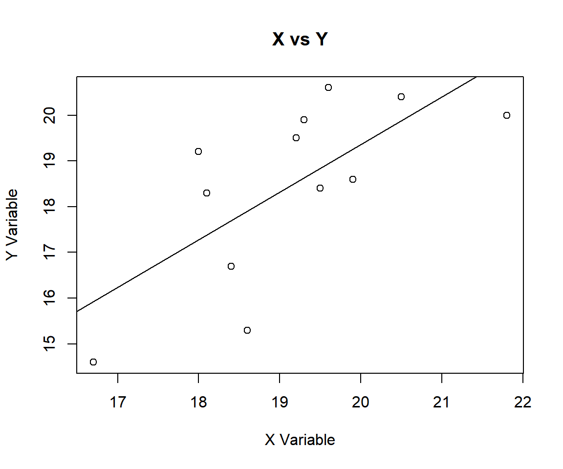
Spearman’s Rank Correlation Coefficient Test X vs Y in R
For the following null hypothesis \(H_0\), and alternative hypothesis \(H_1\), with the level of significance \(\alpha=0.05\).
\(H_0:\) there is no rank correlation between \(x\) and \(y\) (\(\rho_s = 0\)).
\(H_1:\) there is a rank correlation between \(x\) and \(y\) (\(\rho_s \neq 0\), hence the default two-sided).
The cor.test() function has the default
alternative as "two.sided", hence, you do not need to specify
the "alternative" argument in this case.
Or:
    Spearman's rank correlation rho

data:  data_x and data_y
S = 82, p-value = 0.01211
alternative hypothesis: true rho is not equal to 0
sample estimates:
      rho
0.7132867
The sample rank correlation coefficient, \(r_s\), is 0.7132867,
The estimated sum of squared difference in ranks, \(S\), is 82,
the p-value, \(p\), is 0.01211.
Interpretation:
- P-value: With the p-value (\(p = 0.01211\)) being less than the level of significance 0.05, we reject the null hypothesis that the population rank correlation coefficient is equal to 0.
3 Two-tailed Spearman’s Rank Correlation Coefficient Test in R
Using the mtcars data from the "datasets" package with 10 sample observations from 32 rows below:
                     mpg cyl  disp  hp drat    wt  qsec vs am gear carb
Mazda RX4           21.0   6 160.0 110 3.90 2.620 16.46  0  1    4    4
Valiant             18.1   6 225.0 105 2.76 3.460 20.22  1  0    3    1
Merc 280            19.2   6 167.6 123 3.92 3.440 18.30  1  0    4    4
Merc 450SL          17.3   8 275.8 180 3.07 3.730 17.60  0  0    3    3
Lincoln Continental 10.4   8 460.0 215 3.00 5.424 17.82  0  0    3    4
Chrysler Imperial   14.7   8 440.0 230 3.23 5.345 17.42  0  0    3    4
AMC Javelin         15.2   8 304.0 150 3.15 3.435 17.30  0  0    3    2
Porsche 914-2       26.0   4 120.3  91 4.43 2.140 16.70  0  1    5    2
Ford Pantera L      15.8   8 351.0 264 4.22 3.170 14.50  0  1    5    4
Volvo 142E          21.4   4 121.0 109 4.11 2.780 18.60  1  1    4    2
For “drat” as the \(x\) group versus “qsec” as the \(y\) group.
For the following null hypothesis \(H_0\), and alternative hypothesis \(H_1\), with the level of significance \(\alpha=0.1\).
\(H_0:\) there is no rank correlation between \(x\) and \(y\) (\(\rho_s = 0\)).
\(H_1:\) there is a rank correlation between \(x\) and \(y\) (\(\rho_s \neq 0\), hence the default two-sided).
Warning in cor.test.default(mtcars$drat, mtcars$qsec, alternative =
"two.sided", : Cannot compute exact p-value with ties
    Spearman's rank correlation rho

data:  mtcars$drat and mtcars$qsec
S = 4954.8, p-value = 0.617
alternative hypothesis: true rho is not equal to 0
sample estimates:
       rho
0.09186863
The warning is because there are ties in the data. Hence, p-value is based on \(t\)-statistics not AS Algorithm
Interpretation:
- P-value: With the p-value (\(p = 0.617\)) being greater than the level of significance 0.1, we fail to reject the null hypothesis that the population rank correlation coefficient is equal to 0.
With continuity correction:
cor.test(mtcars$drat, mtcars$qsec,
         alternative = "two.sided",
         method = "spearman",
         continuity = TRUE)
Warning in cor.test.default(mtcars$drat, mtcars$qsec, alternative =
"two.sided", : Cannot compute exact p-value with ties
    Spearman's rank correlation rho

data:  mtcars$drat and mtcars$qsec
S = 4954.8, p-value = 0.6164
alternative hypothesis: true rho is not equal to 0
sample estimates:
       rho
0.09186863
This gives a slightly different p-value as continuity correction is applied, and the rank correlation coefficient is slightly adjusted.
Interpretation:
- P-value: With the p-value (\(p = 0.6164\)) being greater than the level of significance 0.1, we fail to reject the null hypothesis that the population rank correlation coefficient is equal to 0.
4 One-tailed Spearman’s Rank Correlation Coefficient Test in R
Right Tailed Test
Using the mtcars data from the "datasets" package above.
For “disp” as the \(x\) group versus “hp” as the \(y\) group.
For the following null hypothesis \(H_0\), and alternative hypothesis \(H_1\), with the level of significance \(\alpha=0.05\).
\(H_0:\) there is no rank correlation between \(x\) and \(y\) (\(\rho_s = 0\)).
\(H_1:\) there is a positive rank correlation between \(x\) and \(y\) (\(\rho_s > 0\), hence one-sided).
Warning in cor.test.default(mtcars$disp, mtcars$hp, alternative = "greater", :
Cannot compute exact p-value with ties
    Spearman's rank correlation rho

data:  mtcars$disp and mtcars$hp
S = 812.71, p-value = 3.396e-10
alternative hypothesis: true rho is greater than 0
sample estimates:
      rho
0.8510426
Interpretation:
- P-value: With the p-value (\(p = 3.396e-10\)) being less than the level of significance 0.05, we reject the null hypothesis that the population rank correlation coefficient is equal to 0.
Left Tailed Test
Using the mtcars data from the "datasets" package above.
For “mpg” as the \(x\) group versus “wt” as the \(y\) group.
For the following null hypothesis \(H_0\), and alternative hypothesis \(H_1\), with the level of significance \(\alpha=0.1\).
\(H_0:\) the population rank correlation coefficient is equal to 0 (\(\rho_s = 0\)).
\(H_1:\) there is a negative rank correlation between \(x\) and \(y\) (\(\rho_s < 0\), hence one-sided).
Warning in cor.test.default(mtcars$mpg, mtcars$wt, alternative = "less", :
Cannot compute exact p-value with ties
    Spearman's rank correlation rho

data:  mtcars$mpg and mtcars$wt
S = 10292, p-value = 7.438e-12
alternative hypothesis: true rho is less than 0
sample estimates:
      rho
-0.886422
Interpretation:
- P-value: With the p-value (\(p = 7.438e-12\)) being less than the level of significance 0.1, we reject the null hypothesis that the population rank correlation coefficient is equal to 0.
5 Spearman’s Rank Correlation Coefficient Test: Estimate, Test Statistics & P-value in R
Here for a Spearman’s rank correlation coefficient test, we show how
to get the estimate (or rank correlation), test statistics (and t-value)
and p-values from the cor.test() function in R, or by
written code.
data_x = mtcars$disp; data_y = mtcars$wt
cor_object = cor.test(data_x, data_y,
                      alternative = "two.sided",
                      method = "spearman")
Warning in cor.test.default(data_x, data_y, alternative = "two.sided", method =
"spearman"): Cannot compute exact p-value with ties
    Spearman's rank correlation rho

data:  data_x and data_y
S = 558.11, p-value = 3.346e-12
alternative hypothesis: true rho is not equal to 0
sample estimates:
      rho
0.8977064
To get the estimate or rank correlation:
\[ r_s = \frac{\sum ^n _{i=1}[r(x_i) - \bar r(x)][r(y_i) - \bar r(y)]}{\sqrt{\sum ^n _{i=1}[r(x_i) - \bar r(x)]^2} \sqrt{\sum ^n _{i=1}[r(y_i) - \bar r(y)]^2}}\]
      rho
0.8977064 [1] 0.8977064Same as:
rx = rank(data_x); ry = rank(data_y)
num = sum((rx-mean(rx))*(ry-mean(ry)))
denom1 = sqrt(sum((rx-mean(rx))^2))
denom2 = sqrt(sum((ry-mean(ry))^2))
r = num/(denom1*denom2)
r
[1] 0.8977064To get the test statistic and t-value:
\[S = \frac{(1-r_s)[n(n^2-1)]}{6}.\]
\[t = \frac{r_s}{\sqrt{\frac{1 - r_s^2}{n-2}}}.\]
       S
558.1137 [1] 558.1137Same as:
[1] 558.1137For t-value:
[1] 11.1598To get the p-value:
Two-tailed: For positive test statistic (\(t^+\)), and negative test statistic (\(t^-\)).
\(Pvalue = 2*P(t_{n-2}>t^+)\) or \(Pvalue = 2*P(t_{n-2}<t^-)\).
One-tailed: For right-tail, \(Pvalue = P(t_{n-2}>t)\) or for left-tail, \(Pvalue = P(t_{n-2}<t)\).
[1] 3.346362e-12Same as:
Note that the p-value depends on the \(\text{test statistic}\) (t = 11.1598) and
\(\text{degrees of freedom}\) (30). We
also use the distribution function pt() for the Student’s
t-distribution in R.
[1] 3.346212e-12[1] 3.34634e-12The feedback form is a Google form but it does not collect any personal information.
Please click on the link below to go to the Google form.
Thank You!
Go to Feedback Form
Copyright © 2020 - 2026. All Rights Reserved by Stats Codes