Logistic Regression in R
Here, we discuss logistic regression in R with interpretations, including coefficients, probability of success, odds ratio, AIC and p-values.
Logistic regression is of the binomial family generalized linear model.
Hence, in R, the logistic regression can be performed with the
glm() function from the "stats" package in base
version of R, specifying the binomial() family and the
logit link.
Logistic regression can be used to study the relationship, if they exist, between a Bernoulli or binomial distributed dependent variable \((y)\), and a set of independent variables \((x_1, x_2, \ldots, x_m)\).
The logistic regression is based on the theoretical assumption that:
\[y\sim Bernoulli(p),\]
and \(y\) is connected to \((x_1, x_2, \ldots, x_m)\) through \(p\) with the logit link function:
\[ \log \left(\frac{p}{1-p}\right) = \beta_0 + \beta_1 x_1 + \beta_2 x_2 + \cdots + \beta_m x_m + \varepsilon,\]
where \(\varepsilon\) represents the
error terms. The logistic regression model then estimates the true
coefficients, \(\beta_1, \beta_2, \ldots,
\beta_m\), as \(\widehat \beta_1,
\widehat \beta_2, \ldots, \widehat \beta_m\), and the true
intercept, \(\beta_0\), as \(\widehat \beta_0\).
Then for any \(x_1, x_2, \ldots, x_m\) values, these are
used to predict or estimate the true \(p\), as \(\widehat p\), with the equation below:
\[\widehat p = \frac{\exp\left( \widehat \beta_0 + \widehat \beta_1 x_1 + \widehat \beta_2 x_2 + \cdots + \widehat \beta_m x_m \right)}{1 + \exp\left( \widehat \beta_0 + \widehat \beta_1 x_1 + \widehat \beta_2 x_2 + \cdots + \widehat \beta_m x_m \right)}.\]
See also linear regression and multiple regression.
Sample Steps to Run a Logistic Regression Model:
# Create the data samples for the logistic regression model
# Values are paired based on matching position in each sample

y = c(1, 0, 1, 1, 0, 0,
      0, 1, 1, 0, 1, 0)
x1 = c(5.05, 4.75, 5.03, 5.82, 6.03, 3.59,
       5.55, 4.62, 5.61, 2.85, 7.56, 4.96)
x2 = c(2.79, 3.27, 2.11, 3.03, 3.43, 2.67,
       3.92, 2.53, 3.58, 2.73, 1.22, 3.31)
lgr_data = data.frame(y, x1, x2)
lgr_data

# Run the logistic regression model

model = glm(y ~ x1 + x2, family = binomial())
summary(model)

# Or

model = glm(y ~ x1 + x2, family = binomial(link = "logit"),
            data = lgr_data)
summary(model)
y x1 x2
1 1 5.05 2.79
2 0 4.75 3.27
3 1 5.03 2.11
4 1 5.82 3.03
5 0 6.03 3.43
6 0 3.59 2.67
7 0 5.55 3.92
8 1 4.62 2.53
9 1 5.61 3.58
10 0 2.85 2.73
11 1 7.56 1.22
12 0 4.96 3.31
Call:
glm(formula = y ~ x1 + x2, family = binomial())

Coefficients:
            Estimate Std. Error z value Pr(>|z|)
(Intercept)    3.138      8.104   0.387   0.6986
x1             2.978      1.750   1.702   0.0888 .
x2            -5.907      3.414  -1.730   0.0836 .
---
Signif. codes:  0 '***' 0.001 '**' 0.01 '*' 0.05 '.' 0.1 ' ' 1

(Dispersion parameter for binomial family taken to be 1)

    Null deviance: 16.6355  on 11  degrees of freedom
Residual deviance:  7.1821  on  9  degrees of freedom
AIC: 13.182

Number of Fisher Scoring iterations: 7| Argument | Usage |
| y ~ x1 + x2 +…+ xm | y is the dependent sample, and x1, x2, …, xm are the independent samples |
| y ~ ., data | y is the dependent sample, and "." means all other variables are in the model |
| family = binomial() | Sets to binomial family, the link can be set in (),
default is "logit" |
| link | Set to binomial(link = "logit"), but not required,
default is "logit" |
| data | The dataframe object that contains the dependent and independent variables |
| weights | For binomial variable, with the proportion of success as the
dependent variable: vector of the number of cases for each proportion of success |
Creating Logistic Regression Summary Object and Model Object:
# Create data
x1 = rnorm(1000, 3, 1)
x2 = rnorm(1000, 2.5, 0.7)
xb = 1.5 + 2*x1 - 3*x2
p = exp(xb)/(1+exp(xb))
y = rbinom(1000, 1, p)

# Create logistic regression model summary and model objects
lgr_summary = summary(glm(y ~ x1 + x2,  family = binomial()))
lgr_model = glm(y ~ x1 + x2, family = binomial())
# Extract a component from logistic regression summary object
lgr_summary$coefficients; lgr_summary$coefficients[, 1] Estimate Std. Error z value Pr(>|z|)
(Intercept) 1.843634 0.4382976 4.206352 2.595263e-05
x1 1.944994 0.1412202 13.772777 3.716496e-43
x2 -3.007622 0.2104453 -14.291707 2.464921e-46(Intercept) x1 x2
1.843634 1.944994 -3.007622 (Intercept) x1 x2
1.843634 1.944994 -3.007622 There are more examples in the table below.
| GLM Component | Usage |
| lgr_model$coefficients | The estimated intercept and beta values |
| lgr_model$fitted.values | The predicted probability values |
| lgr_model$linear.predictors | The predicted linear model values |
| lgr_model$residuals | The linear model residuals |
| lgr_model$aic | The Akaike’s An Information Criterion value |
| lgr_model$null.deviance | The null model’s deviance |
| lgr_model$deviance | The model’s deviance |
| lgr_model$df.residual | The model’s residual degrees of freedom |
| lgr_model$df.null | The null model’s residual degrees of freedom |
| lgr_model$model | The model dataframe |
| lgr_summary$coefficients | The estimated intercept and beta values: their standard error, z-value and p-value |
| lgr_summary$aic | The Akaike’s An Information Criterion value |
| lgr_summary$null.deviance | The null model’s deviance |
| lgr_summary$deviance | The model’s deviance |
| lgr_summary$df.residual | The model’s residual degrees of freedom |
| lgr_summary$df.null | The null model’s residual degrees of freedom |
1 Logistic Regression with Single Variable in R
Using the "mtcars" data from the "datasets" package with 10 sample rows below:
                    mpg cyl  disp  hp drat    wt  qsec vs am gear carb
Mazda RX4          21.0   6 160.0 110 3.90 2.620 16.46  0  1    4    4
Datsun 710         22.8   4 108.0  93 3.85 2.320 18.61  1  1    4    1
Valiant            18.1   6 225.0 105 2.76 3.460 20.22  1  0    3    1
Cadillac Fleetwood 10.4   8 472.0 205 2.93 5.250 17.98  0  0    3    4
Chrysler Imperial  14.7   8 440.0 230 3.23 5.345 17.42  0  0    3    4
Camaro Z28         13.3   8 350.0 245 3.73 3.840 15.41  0  0    3    4
Fiat X1-9          27.3   4  79.0  66 4.08 1.935 18.90  1  1    4    1
Porsche 914-2      26.0   4 120.3  91 4.43 2.140 16.70  0  1    5    2
Maserati Bora      15.0   8 301.0 335 3.54 3.570 14.60  0  1    5    8
Volvo 142E         21.4   4 121.0 109 4.11 2.780 18.60  1  1    4    2
NOTE: The dependent variable is "vs", which is engine type: 0 = V-shaped, and 1 = straight. The independent variable is "qsec", the time to reach a quarter mile.
1.1 Check for Relationship
Use a box plot to visually check for a relationship.
qsec = mtcars$qsec
vs = mtcars$vs
boxplot(qsec ~ vs,
     main = "Box Plot for Logistic Regression in R")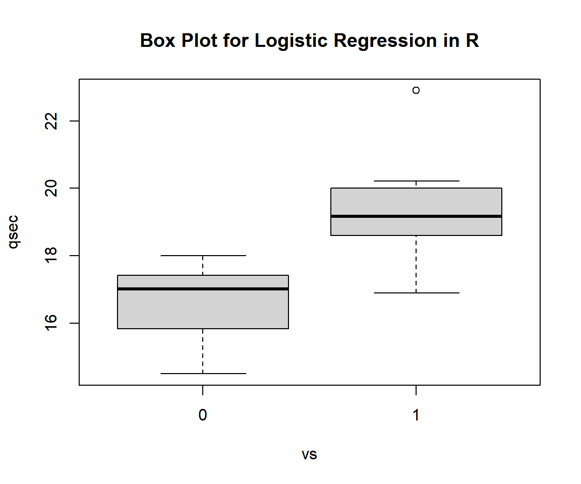
Box Plot for Logistic Regression in R
The appearance of the boxplot suggests a strong relationship between "vs" and "qsec". The box for "1" or "straight" shaped engine appears significantly higher.
1.2 Run the Logistic Regression
Run the single variable logistic regression model using the
glm() function and family = binomial(), and
print the results using the summary() function.
Or:
Call:
glm(formula = vs ~ qsec, family = binomial(), data = mtcars)

Coefficients:
            Estimate Std. Error z value Pr(>|z|)
(Intercept)  -56.361     21.455  -2.627  0.00862 **
qsec           3.123      1.192   2.619  0.00881 **
---
Signif. codes:  0 '***' 0.001 '**' 0.01 '*' 0.05 '.' 0.1 ' ' 1

(Dispersion parameter for binomial family taken to be 1)

    Null deviance: 43.860  on 31  degrees of freedom
Residual deviance: 14.076  on 30  degrees of freedom
AIC: 18.076

Number of Fisher Scoring iterations: 7
1.3 Interpretation of the Results
- Coefficients:
- The estimated intercept (\(\widehat \beta_0\)) is \(\text{summary(model)\$coefficients[1, 1]}\) \(= -56.36123\).
- The estimated coefficient for \(x\) (\(\widehat \beta_1\)) is \(\text{summary(model)\$coefficients[2, 1]}\) \(= 3.1229\).
- P-values:
For level of significance, \(\alpha = 0.05\).- The p-value for the independent variable, \(x\) ("qsec"), is \(\text{summary(model)\$coefficients[2, 4]}\)
\(= 0.0088134\). Since the p-value is
less than \(0.05\), we say that the
independent variable is a statistically significant predictor of the
dependent variable \(y\) ("vs").
If the p-value were higher than the chosen level of significance, we would have concluded otherwise.
- The p-value for the independent variable, \(x\) ("qsec"), is \(\text{summary(model)\$coefficients[2, 4]}\)
\(= 0.0088134\). Since the p-value is
less than \(0.05\), we say that the
independent variable is a statistically significant predictor of the
dependent variable \(y\) ("vs").
- AIC:
The AIC value is \(\text{summary(model)\$aic}\) \(= 18.076\).
When comparing the model to other models for predicting "vs" based on the same data, the model with a lower AIC is better.
1.4 Odds and Odds Ratio
With \(p_{vs} = \text{Probability(vs = 1)}\).
\(\log \left(\frac{\widehat p_{vs}}{1- \widehat p_{vs}} \right)\) \(= \widehat \beta_0 + \widehat \beta_1 \times qsec\) \(= -56.36123 + 3.1229 \times qsec.\)
Odds:
Hence, the odds, \(\frac{\widehat p_{vs}}{1 - \widehat p_{vs}}\), is \(\exp \left( -56.36123 + 3.1229 \times qsec \right).\)
Therefore, for 1 unit increase in \(x\) ("qsec"), the odds is multiplied by (or increases by a factor of) \(\exp (3.1229)\) = \(22.712\).
Odds Ratio:
For two different values of "qsecs", \(x_1\) and \(x_2\), the odds ratio, \(\left(\frac{\widehat p_{vs\_x2}}{1 - \widehat p_{vs\_x2}}\right)/\left(\frac{\widehat p_{vs\_x1}}{1 - \widehat p_{vs\_x1}}\right)\), is \(\exp (3.1229 \times x_2) / \exp (3.1229 \times x_1).\)
1.5 Prediction and Estimation
With \(p_{vs} = \text{Probability(vs = 1)}\).
\(\widehat p_{vs}\) \(= \frac{\exp (-56.36123 \; + \; 3.1229 \times qsec)}{1 + \exp (-56.36123 \; + \; 3.1229 \times qsec)}\).
For example, for \(x = 18\) (qsec = 18), \(\widehat p_{vs}\) \(= \frac{\exp (-56.36123 \; + \; 3.1229 \times 18)}{1 \; + \; \exp (-56.36123 \; + \; 3.122896 \times 18)}\) \(= \frac{\exp (-0.149)}{1 \; + \; \exp (-0.149)}\) \(= 0.463\).
With \(\widehat p_{vs} = 0.463\), which is less than \(0.5\), we should predict \(vs = 0\), that is, engine is V-shaped.
2 Logistic Regression with Categorical Independent Variable in R
Using the same "mtcars" data from the "datasets" package above.
NOTE: The dependent variable is "am", which is transmission type: 0 = automatic, and 1 = manual. The categorical independent variable is "cyl", which is number of cylinders category: 4, 6, or 8.
   cyl
am   4  6  8
  0  3  4 12
  1  8  3  2
The table of "am" versus "cyl" shows that the higher the "cyl", the more likely it is that "am = 0", and the lower the "cyl", the more likely it is that "am = 1".
Run the Logistic Regression
Run the categorical independent variable logistic regression model
using the glm() function and
family = binomial(), and print the results using the
summary() function.
Setting "cyl" as a factor helps treat it as a categorical variable instead of a numeric variable.
Or:
Call:
glm(formula = am ~ factor(cyl), family = binomial(), data = mtcars)

Coefficients:
             Estimate Std. Error z value Pr(>|z|)
(Intercept)    0.9808     0.6770   1.449   0.1474
factor(cyl)6  -1.2685     1.0206  -1.243   0.2139
factor(cyl)8  -2.7726     1.0206  -2.717   0.0066 **
---
Signif. codes:  0 '***' 0.001 '**' 0.01 '*' 0.05 '.' 0.1 ' ' 1

(Dispersion parameter for binomial family taken to be 1)

    Null deviance: 43.230  on 31  degrees of freedom
Residual deviance: 33.935  on 29  degrees of freedom
AIC: 39.935

Number of Fisher Scoring iterations: 4
Interpretation of the Results
- Coefficients:
- The estimated coefficient for "4 cylinders" is the intercept, \(\text{summary(model)\$coefficients[1, 1]}\) \(= 0.98083\).
- The estimated effect of "6 cylinders" versus "4 cylinders" is \(\text{summary(model)\$coefficients[2, 1]}\) \(= -1.26851\).
- The estimated effect of "8 cylinders" versus "4 cylinders" is \(\text{summary(model)\$coefficients[3, 1]}\) \(= -2.77259\).
- P-values:
For level of significance, \(\alpha = 0.05\).- The p-value for the intercept ("4 cylinders"), is \(\text{summary(model)\$coefficients[1, 4]}\) \(= 0.1474\). Since the p-value is greater than \(0.05\), we say that the log(odds of automatic transmission = "1") with "4 cylinders" is NOT statistically different from 0, or the probability of success (automatic transmission = "1") with "4 cylinders" is NOT statistically different from 0.5 (50-50 guess).
- The p-value for "6 cylinders" effect is \(\text{summary(model)\$coefficients[2, 4]}\) \(= 0.21391\). Since the p-value is greater than \(0.05\), we say that the log(odds of automatic transmission = "1") for "6 cylinders" is NOT statistically significantly different from that of "4 cylinders", or the probability of success (automatic transmission = "1") with "6 cylinders" is NOT statistically different from that of "4 cylinders".
- The p-value for "8 cylinders" effect is \(\text{summary(model)\$coefficients[3, 4]}\) \(= 0.0066\). Since the p-value is less than \(0.05\), we say that the log(odds of automatic transmission = "1") for "8 cylinders" is statistically significantly different from that of "4 cylinders", or the probability of success (automatic transmission = "1") with "8 cylinders" is statistically different from that of "4 cylinders".
- AIC:
The AIC value is \(\text{summary(model)\$aic}\) \(= 39.935\).
When comparing the model to other models for predicting "am" based on the same data, the model with a lower AIC is better.
Odds and Odds Ratio
With \(p_{am} = \text{Probability(am = 1)}\).
\(\log \left(\frac{\widehat p_{am}}{1- \widehat p_{am}} \right)\) \(= \widehat \beta_{intercept} + \widehat \beta_{category}.\)
Hence, the odds, \(\frac{\widehat p_{am}}{1 - \widehat p_{am}}\), are:
"4 cylinders": \(\frac{\widehat p_{am}}{1 - \widehat p_{am}}\) \(= \exp \left( 0.98083 \right)\) \(= 2.667.\)
"6 cylinders": \(\frac{\widehat p_{am}}{1 - \widehat p_{am}}\) \(= \exp \left( 0.98083 + (-1.26851) \right)\) \(=\exp \left( -0.2877 \right)\) \(= 0.75.\)
"8 cylinders": \(\frac{\widehat p_{am}}{1 - \widehat p_{am}}\) \(= \exp \left( 0.98083 + (-2.77259) \right)\) \(=\exp \left( -1.7918 \right)\) \(= 0.167.\)
Also, the odds ratio, \(\left(\frac{\widehat p_{am\_*cyl}}{1 - \widehat p_{am\_*cyl}}\right)/\left(\frac{\widehat p_{am\_4cyl}}{1 - \widehat p_{am\_4cyl}}\right)\), are:
"6 cylinders" versus "4 cylinders": \(\left(\frac{\widehat p_{am\_6cyl}}{1 - \widehat p_{am\_6cyl}}\right)/\left(\frac{\widehat p_{am\_4cyl}}{1 - \widehat p_{am\_4cyl}}\right)\) \(= \exp \left(-1.26851\right)\) \(= 0.281.\)
"8 cylinders" versus "4 cylinders": \(\left(\frac{\widehat p_{am\_8cyl}}{1 - \widehat p_{am\_8cyl}}\right)/\left(\frac{\widehat p_{am\_4cyl}}{1 - \widehat p_{am\_4cyl}}\right)\) \(= \exp \left(-2.77259\right)\) \(= 0.063.\)
Prediction and Estimation
With \(p_{am} = \text{Probability(am = 1)}\).
"4 cylinders": \(\widehat p_{am}\) \(= \frac{\exp \left( 0.9808 \right)}{1 \; + \; \exp \left( 0.9808 \right)}\) \(= 0.727.\)
"6 cylinders": \(\widehat p_{am}\) \(=\frac{\exp \left( -0.2877 \right)}{1 \; + \; \exp \left( -0.2877 \right)}\) \(= 0.429.\)
"8 cylinders": \(\widehat p_{am}\) \(=\frac{\exp \left( -1.7918 \right)}{1 \; + \; \exp \left( -1.7918 \right)}\) \(= 0.143.\)
Hence, we predict \(am = 1\) (automatic transmission = "1") for "4 cylinders" since \(0.727\) is greater than \(0.5\).
Also, we predict \(am = 0\) (automatic transmission = "0") for "6 cylinders" and "8 cylinders" since \(0.429\) and \(0.143\) are less than \(0.5\).
3 Logistic Regression with Numeric & Categorical Independent Variables in R
Using the same "mtcars" data from the "datasets" package above.
NOTE: The dependent variable is "vs", which is engine type: 0 = V-shaped, and 1 = straight. The independent variables are "wt", weight in 1000lbs, and "am", which is transmission type: 0 = automatic, and 1 = manual.
Run the Logistic Regression
Run the logistic regression model with numeric and categorical
independent variables using the glm() function and
family = binomial(), and print the results using the
summary() function.
Setting "am" as a factor helps treat it as a categorical variable instead of a numeric variable.
vs = mtcars$vs
wt = mtcars$wt
am = factor(mtcars$am)
model = glm(vs ~ wt + am, family = binomial())
summary(model)
Or:
Call:
glm(formula = vs ~ wt + factor(am), family = binomial(), data = mtcars)

Coefficients:
            Estimate Std. Error z value Pr(>|z|)
(Intercept)   21.751      8.433   2.579  0.00991 **
wt            -6.330      2.425  -2.611  0.00904 **
factor(am)1   -6.133      2.700  -2.272  0.02312 *
---
Signif. codes:  0 '***' 0.001 '**' 0.01 '*' 0.05 '.' 0.1 ' ' 1

(Dispersion parameter for binomial family taken to be 1)

    Null deviance: 43.860  on 31  degrees of freedom
Residual deviance: 21.532  on 29  degrees of freedom
AIC: 27.532

Number of Fisher Scoring iterations: 7
Interpretation of the Results
- Coefficients:
- The estimated coefficient for "(am)0 - automatic" is the intercept, \(\text{summary(model)\$coefficients[1, 1]}\) \(= 21.75053\).
- The estimated coefficient for "wt" is \(\text{summary(model)\$coefficients[2, 1]}\) \(= -6.32969\).
- The estimated effect of "(am)1 - manual" versus "(am)0 - automatic" is \(\text{summary(model)\$coefficients[3, 1]}\) \(= -6.13349\).
- P-values:
For level of significance, \(\alpha = 0.05\).- The p-value for the intercept ("(am)0 - automatic"), is \(\text{summary(model)\$coefficients[1, 4]}\) \(= 0.00991\). Since the p-value is less than \(0.05\), we say that the log(odds of V-shaped engine = "1") with "(am)0 - automatic" and "wt = 0" is statistically different from 0, or the probability of success (V-shaped engine = "1") with "(am)0 - automatic" and "wt = 0" is statistically different from 0.5 (50-50 guess).
- The p-value for "wt" is \(\text{summary(model)\$coefficients[2, 4]}\) \(= 0.00904\). Since the p-value is less than \(0.05\), we say that "wt" is a statistically significant predictor of the log(odds of V-shaped engine = "1") or probability of success (V-shape = "1”).
- The p-value for "(am)1 - manual" effect is \(\text{summary(model)\$coefficients[3, 4]}\) \(= 0.02312\). Since the p-value is less than \(0.05\), we say that, for any given "wt" value, the log(odds of V-shaped engine = "1") for "(am)1 - manual" is statistically significantly different from that of "(am)0 - automatic". Also, for any given "wt" value, the probability of success (V-shaped engine = "1") with "(am)1 - manual" is statistically different from that of "(am)0 - automatic".
- AIC:
The AIC value is \(\text{summary(model)\$aic}\) \(= 27.532\).
When comparing the model to other models for predicting "vs" based on the same data, the model with a lower AIC is better.
Odds
With \(p_{vs} = \text{Probability(vs = 1)}\).
\(\log \left(\frac{\widehat p_{vs}}{1- \widehat p_{vs}} \right)\) \(= \widehat \beta_{intercept} +\beta_{category} + \widehat \beta_{weight} \times weight.\)
Hence, the odds, \(\frac{\widehat p_{vs}}{1 - \widehat p_{vs}}\), are:
For "(am)0 - automatic": \(\frac{\widehat p_{vs}}{1 - \widehat p_{vs}}\) \(= \exp \left( 21.75053 + (-6.32969) \times weight \right).\)
For "(am)1 - manual": \(\frac{\widehat p_{vs}}{1 - \widehat p_{vs}}\) \(= \exp \left( 21.75053 + (-6.13349) + (-6.32969) \times weight \right).\)
Hence, for 3000lbs of weight (wt = 3), the odds, \(\frac{\widehat p_{vs}}{1 - \widehat p_{vs}}\), are:
For "(am)0 - automatic": \(\frac{\widehat p_{vs}}{1 - \widehat p_{vs}}\) \(= \exp \left( 21.7505 + (-6.32969) \times 3 \right)\) \(=\exp \left( 2.76144 \right)\) \(= 15.823.\)
For "(am)1 - manual": \(\frac{\widehat p_{vs}}{1 - \widehat p_{vs}}\) \(= \exp \left( 21.75053 + (-6.13349) + (-6.32969) \times 3 \right)\) \(=\exp \left( -3.372 \right)\) \(= 0.034.\)
Prediction and Estimation
Similarly, for 3000lbs of weight (wt = 3), \(p_{vs} = \text{Probability(vs = 1)}\) are:
For "(am)0 - automatic": \(\widehat p_{vs}\) \(= \frac{\exp \left(2.76144 \right)}{1 \; + \; \exp \left(2.76144 \right)}\) \(= 0.941.\)
For "(am)1 - manual": \(\widehat p_{vs}\) \(= \frac{\exp \left(-3.372 \right)}{1 \; + \; \exp \left(-3.372 \right)}\) \(= 0.0332.\)
Hence, we predict \(vs = 1\) (V-shaped = "1") for "(am)0 - automatic" since \(0.941\) is greater than \(0.5\).
Also, we predict \(vs = 0\) (V-shaped = "0") for "(am)1 - manual" since \(0.0332\) is less than \(0.5\).
4 Logistic Regression with Multiple Independent Variables in R
Using the same "mtcars" data from the "datasets" package above.
NOTE: The dependent variable is "am", which is transmission type: 0 = automatic, and 1 = manual. The independent variables are "disp" (displacement (cu.in.)), and "hp" (horsepower).
Run the Logistic Regression
Run the logistic regression model with multiple independent variables
using the glm() function and
family = binomial(), and print the results using the
summary() function.
am = mtcars$am
disp = mtcars$disp
hp = mtcars$hp
model = glm(am ~ disp + hp, family = binomial())
summary(model)
Or:
Call:
glm(formula = am ~ disp + hp, family = binomial(), data = mtcars)

Coefficients:
            Estimate Std. Error z value Pr(>|z|)
(Intercept)  1.40342    1.36757   1.026   0.3048
disp        -0.09518    0.04800  -1.983   0.0474 *
hp           0.12170    0.06777   1.796   0.0725 .
---
Signif. codes:  0 '***' 0.001 '**' 0.01 '*' 0.05 '.' 0.1 ' ' 1

(Dispersion parameter for binomial family taken to be 1)

    Null deviance: 43.230  on 31  degrees of freedom
Residual deviance: 16.713  on 29  degrees of freedom
AIC: 22.713

Number of Fisher Scoring iterations: 8
b0 = summary(model)$coefficients[1,1]
b1 = summary(model)$coefficients[2,1]
b2 = summary(model)$coefficients[3,1]
am = mtcars$am; disp = mtcars$disp; hp = mtcars$hp
plot(disp, hp, col = (am + 2),
main = "Plot of Actuals versus Decision Boundary")
segments(x0 = (-b0/b1 - (b2*min(hp))/b1), y0 = min(hp),
x1 = (-b0/b1 - (b2*max(hp))/b1), y1 = max(hp),
col = "blue")
legend("topleft",
c("0", "1"),
fill = c("red", "green"))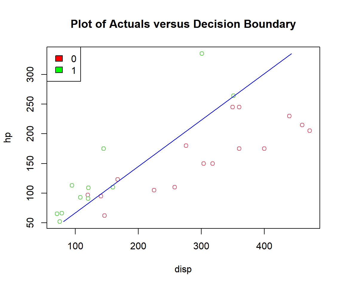
Plot of Logistic Regression Decision Boundary in R
Above, the greens are "1", and the reds are "0".
Interpretation of the Results
- Coefficients:
- The estimated coefficient for "disp" is \(\text{summary(model)\$coefficients[2, 1]}\) \(= -0.09518\).
- The estimated coefficient for "hp" is \(\text{summary(model)\$coefficients[3, 1]}\) \(= 0.1217\).
- P-values:
For level of significance, \(\alpha = 0.05\).- The p-value for "disp" is \(\text{summary(model)\$coefficients[2, 4]}\) \(= 0.04739\). Since the p-value is less than \(0.05\), we say that "disp" is a statistically significant predictor of the dependent variable \(y\) ("am") or probability of success (automatic transmission = "1").
- The p-value for "hp" is \(\text{summary(model)\$coefficients[3, 4]}\) \(= 0.07254\). Since the p-value is greater than \(0.05\), we say that "hp" is NOT a statistically significant predictor of the dependent variable \(y\) ("am").
- AIC:
The AIC value is \(\text{summary(model)\$aic}\) \(= 22.713\).
When comparing the model to other models for predicting "am" based on the same data, the model with a lower AIC is better.
Odds
With \(p_{am} = \text{Probability(am = 1)}\).
\(\log \left(\frac{\widehat p_{am}}{1- \widehat p_{am}} \right)\) \(= \widehat \beta_{intercept} + \widehat \beta_{disp} \times disp + \widehat \beta_{hp} \times hp.\)
Hence, the odds, \(\frac{\widehat p_{am}}{1 - \widehat p_{am}}\), is \(\exp \left( 1.40342 + -0.09518 \times disp + 0.1217 \times hp \right).\)
Therefore, for 1 unit increase in \(x_1\) ("disp"), the odds is multiplied by \(\exp (-0.09518)\) \(= 0.909\).
Also, for 1 unit increase in \(x_2\) ("hp"), the odds is multiplied by \(\exp (0.1217)\) \(= 1.129\).
Prediction and Estimation
The estimated \(p_{am} = \text{Probability(am = 1)}\) is, \(\widehat p_{am}\) \(= \frac{\exp (1.40342 \; + \; (-0.09518) \times disp \; + \; 0.1217 \times hp)}{1 \; + \; \exp (1.40342 \; + \; (-0.09518) \times disp \; + \; 0.1217 \times hp)}\).
For example, for \(x_1 = 240\) (240
cu. in. of displacement), and \(x_2 =
160\) (160 horsepower):
\(\widehat
p_{am}\) \(= \frac{\exp (1.40342 \; +
\; (-0.09518) \times 240 \; + \; 0.1217 \times 160)}{1 \; + \; \exp
(1.40342 \; + \; (-0.09518) \times 240 \; + \; 0.1217 \times
160)}\) \(= \frac{\exp (-1.967)}{1 \; +
\; \exp (-1.967)}\) \(=
0.123\).
With \(\widehat p_{am} = 0.123\), which is less than \(0.5\), we should predict \(am = 0\), that is, transmission is automatic.
The feedback form is a Google form but it does not collect any personal information.
Please click on the link below to go to the Google form.
Thank You!
Go to Feedback Form
Copyright © 2020 - 2026. All Rights Reserved by Stats Codes