Histograms in R
- 1 Create a Simple Histogram in R
- 2 Create Density Histogram with Density Curve in R
- 3 Set Breaks and Widths of Histogram in R
- 4 Set Title, Labels, Limits, Colors, Fonts of a Histogram in R
- 5 Create Histogram from a Frequency Table
- 6 Add Counts on Bars in Histogram in R
- 7 Multiple Histograms in One Plot in R
Here, we show how to make histograms and density histograms in R, and set breaks, widths, title, labels, limits, colors, and fonts.
These are done with the hist() function.
See plots & charts for graphical parameters and other plots and charts.
1 Create a Simple Histogram in R
Enter the data by hand:
Histdata = c(162, 150, 142, 126, 149, 195, 82, 194, 111, 122)
hist(Histdata, main = "Simple Histogram")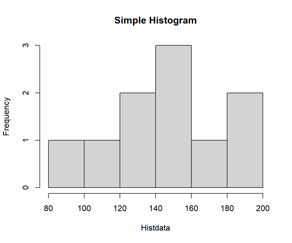
Example 1: Simple Histogram in R
Using a Data Object:
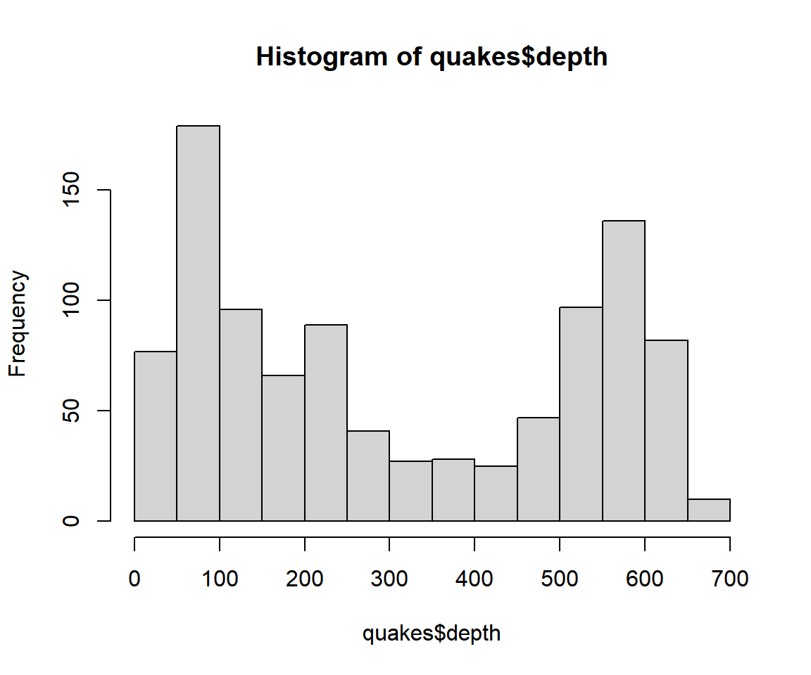
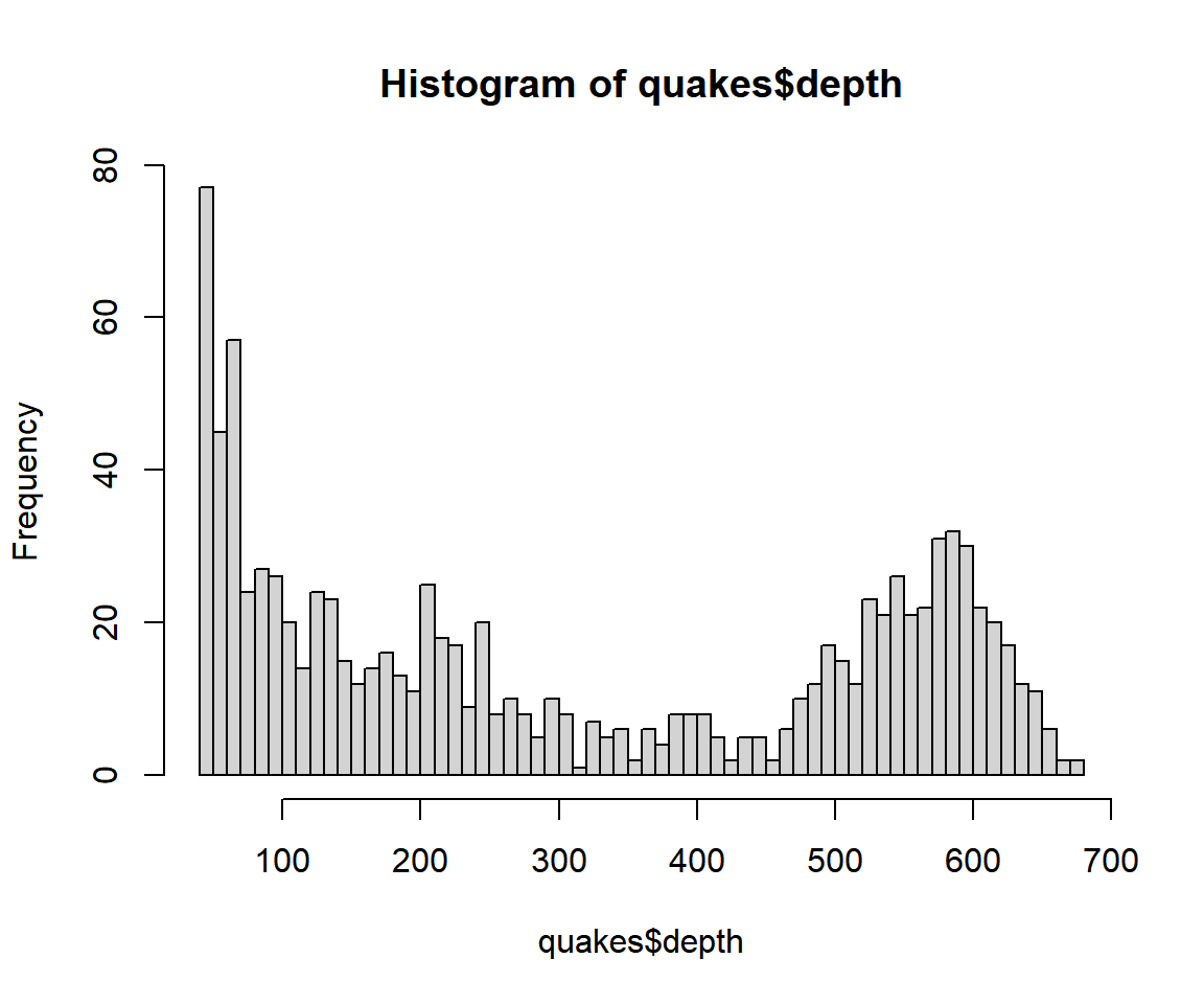
Using the quakes data from the "datasets" package with some sub-setting and filtering.
Sample rows from quakes:
        lat   long depth mag stations
1    -20.42 181.62   562 4.8       41
102  -26.20 178.41   583 4.6       25
285  -17.95 184.68   260 4.4       21
624  -23.78 180.31   518 5.1       71
646  -23.29 184.00   164 4.8       50
849  -22.23 180.48   581 5.0       54
906  -17.44 181.33   545 4.2       37
919  -25.06 182.80   133 4.0       14
935  -20.25 184.75   107 5.6      121
1000 -21.59 170.56 165 6.0 119Or:
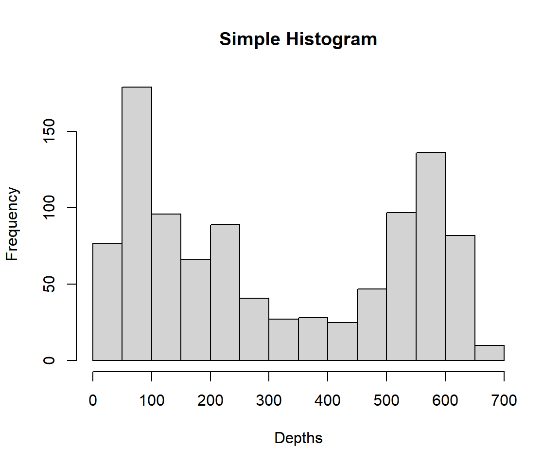
Example 2: Simple Histogram in R
2 Create Density Histogram with Density Curve in R
To make density histogram, specify the "freq" argument as "FALSE".
Use the density() function to specify the curve. The
lines() function adds the curve to the histogram, with the
"lwd" argument used to specify the line width, the higher the thicker
the line. See also density plots
and line types &
widths.
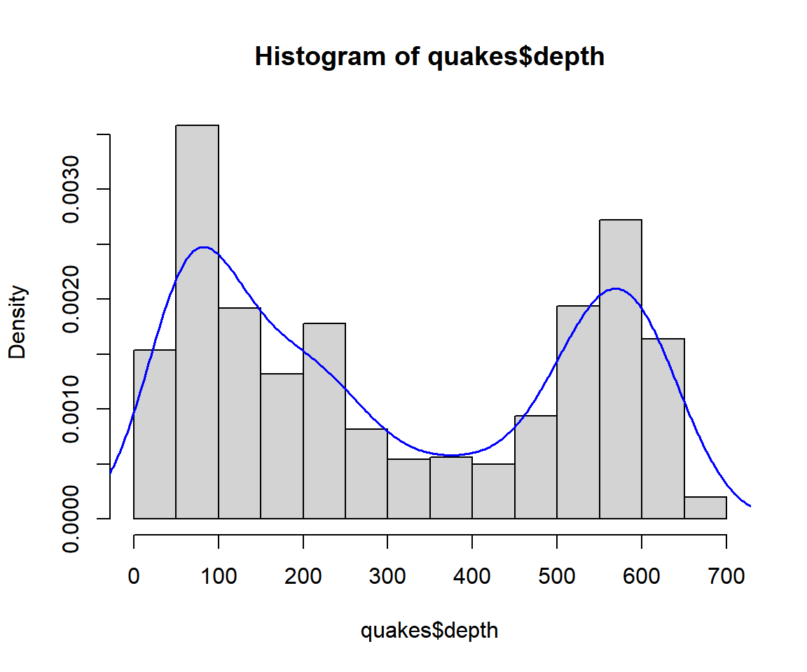
Density Histogram with Density Curve in R
3 Set Breaks and Widths of Histogram in R
Set Histogram to Have Breaks:
This example has 12 breaks. R finds around 12 convenient breaks.
Example 1: Histogram with Breaks Set in R
Similarly for 60 breaks.
Example 2: Histogram with Breaks Set in R
Set Histogram to Have Specific Breaks:
This example has equidistant breaks.
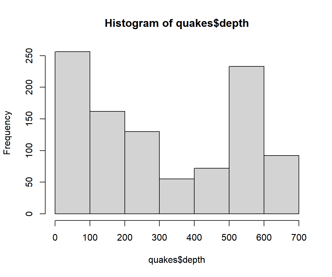
Example 3: Histogram with Breaks Set in R
This example has unequal widths which makes R scale the heights automatically to the density scale.
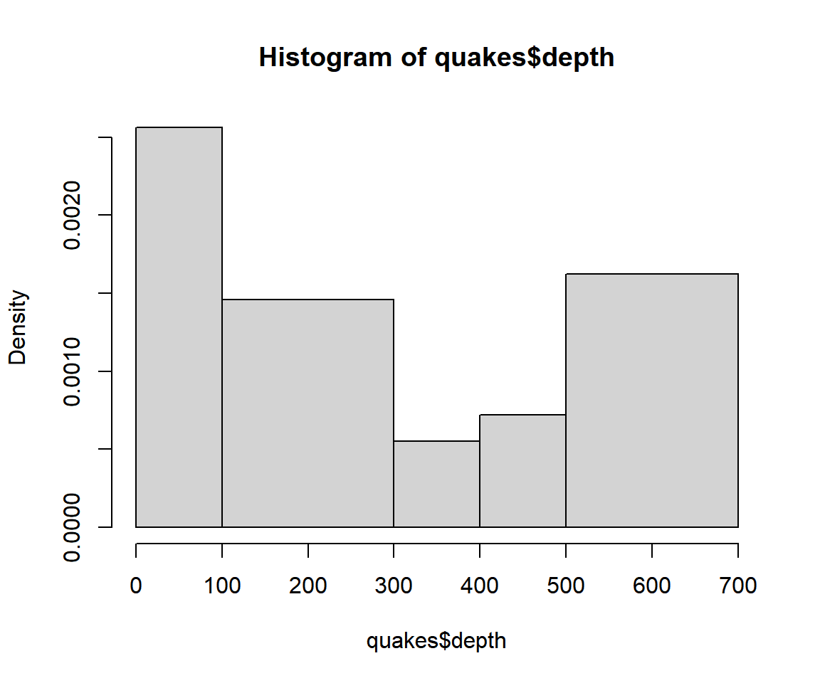
Example 4: Histogram With Breaks Set in R
4 Set Title, Labels, Limits, Colors, Fonts of a Histogram in R
Here we set details such as title (main), x-axis and y-axis labels (xlab, ylab), limits (xlim, ylim), colors (col, border), font types (font), and font sizes (cex). See also setting colors and fonts for more details.
hist(quakes$depth,
     breaks = c(0, 100, 200, 300, 400, 500, 600, 700),
     main = "Histogram of Depths",
     xlab = "Depths (km)",
     ylab = "Frequency of Depths",
     xlim = c(0, 800),
     ylim = c(0, 300),
     col = "green",
     col.main="red", col.lab="blue", col.axis="brown",
     border = "red",
     font=2, font.lab=1, font.main=2,
     cex.main=1.6, cex.lab=1.25, cex.axis=1.2)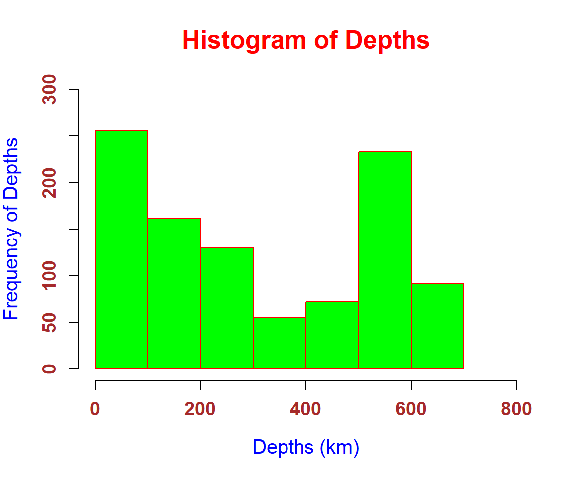
Histogram with Title, Labels, Limits, Colors, Fonts Set in R
5 Create Histogram from a Frequency Table
| Height | Frequency |
| 50-52 | 4 |
| 53-55 | 14 |
| 56-58 | 16 |
| 59-61 | 8 |
Two vectors are to be specified, the breaks, and the density for the heights. Then these will be combined into a list with Class set to "histogram".
breaks = c(50, 53, 56, 59, 61)
counts = c(4, 14, 16, 8)
hist1 = list(breaks=breaks, density=counts)
class(hist1) = "histogram"
plot(hist1, main = "Histogram of Heights",
     xlab = "Heights (inches)",
     ylab = "Frequency of Heights")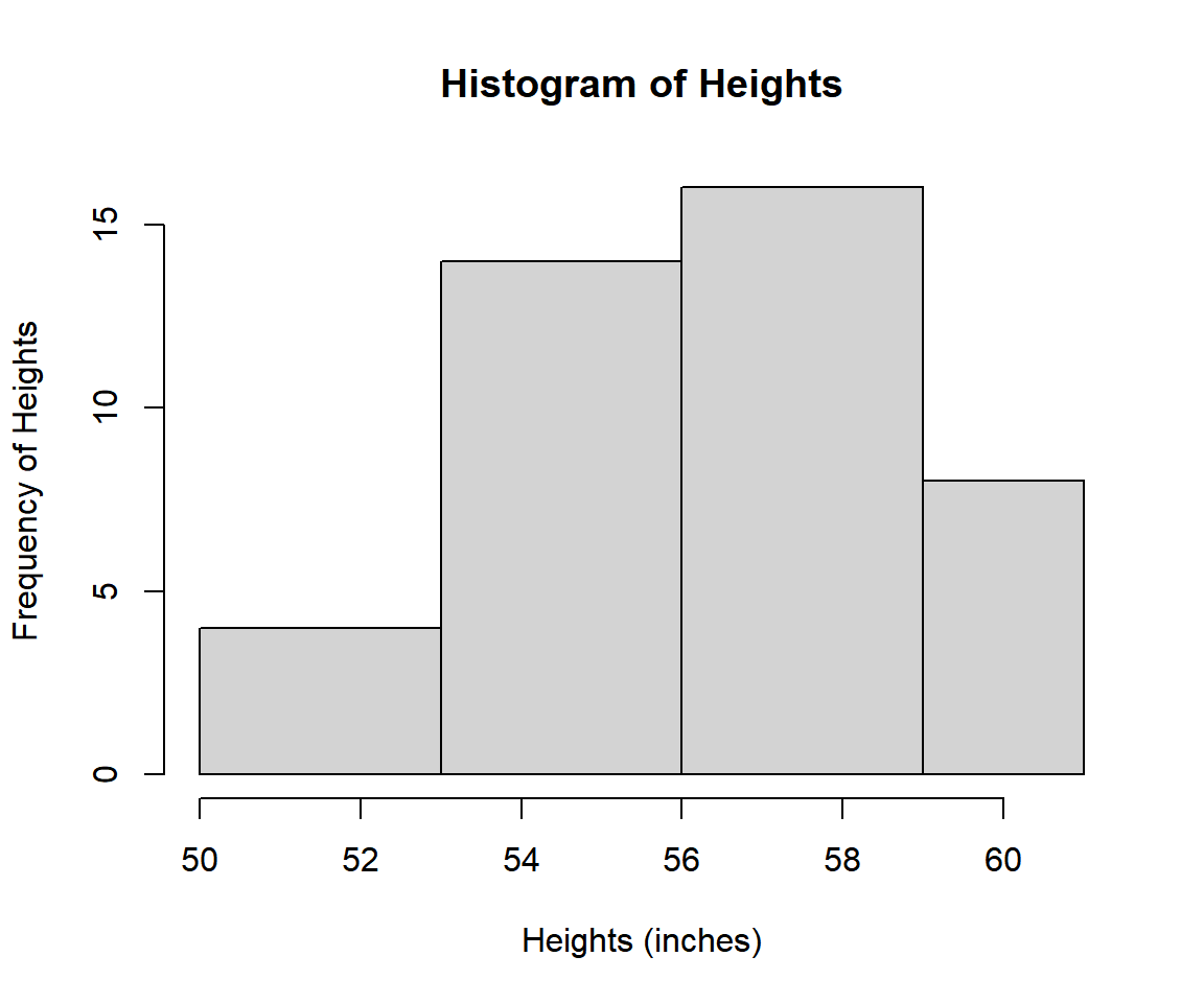
Histogram from Frequency Table in R
For density histogram, instead of setting "density=counts", we will derive the densities and set "density=density".
breaks = c(50, 53, 56, 59, 61)
counts = c(4, 14, 16, 8)
relativefreq = counts/sum(counts)
widths = c(3, 3, 3, 3)
density = relativefreq/widths
hist2 = list(breaks=breaks, density=density)
class(hist2) = "histogram"
plot(hist2, main = "Density Histogram of Heights",
     xlab = "Heights (inches)",
     ylab = "Frequency of Heights")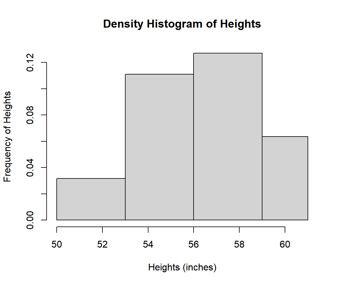
Density Histogram from Frequency Table in R
6 Add Counts on Bars in Histogram in R
To add counts to histogram bars
in R, use the text() function. First assign a name to your
histogram object then add text to the object with the
text() function. The first and second arguments of the text
function are the x and y co-ordinates, while the third are the values to
be printed. The "adj" argument is used to shift the text to a location
of choice.
Example for Frequency Histogram:
hplot1 = hist(quakes$depth,
             breaks = c(0, 100, 200, 300, 400, 500, 600, 700),
             ylim = c(0, 280))
text(hplot1$mids, hplot1$counts, hplot1$counts, adj = c(0.5, -0.5), col = "Green")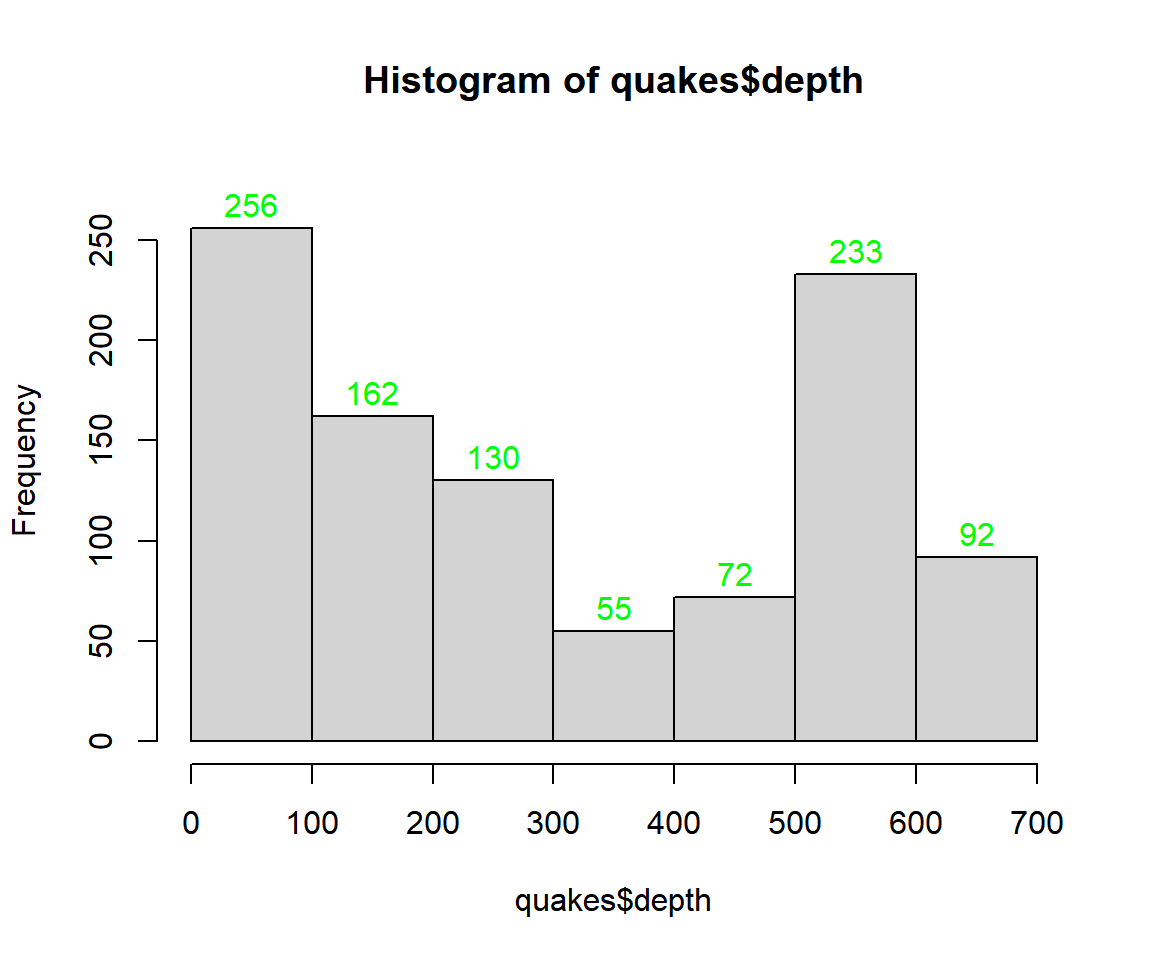
Histogram with Counts on Bars in R
Example for Density Histogram:
hplot2 = hist(quakes$depth,
             breaks = c(0, 100, 300, 400, 500, 700),
             ylim = c(0, 0.004))
text(hplot2$mids, hplot2$density, hplot2$counts, adj = c(0.5, -0.5), col = "Green")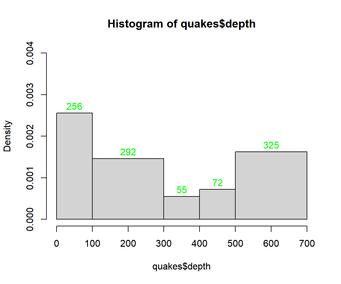
Density Histogram with Counts on Bars in R
7 Multiple Histograms in One Plot in R
To have multiple
histograms in one plot, use the par() function. The
first argument is the number of rows, while the second is the number of
columns. Then make your histograms, and they will be added one after the
other. Details can be added to each histogram as with the examples
above.
For example, for 2 rows and 2 columns use:
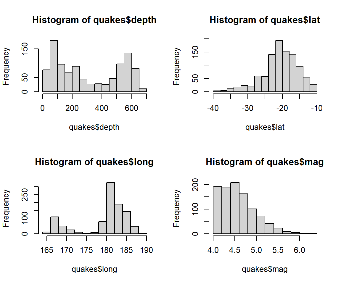
Multiple Histograms in One Plot in R
The feedback form is a Google form but it does not collect any personal information.
Please click on the link below to go to the Google form.
Thank You!
Go to Feedback Form
Copyright © 2020 - 2026. All Rights Reserved by Stats Codes