Chi-squared Contingency Table Tests in R
- 1 Test Statistic for Chi-squared Contingency Table Test in R
- 2 Simple Chi-squared Test of Independence in R
- 3 Chi-squared Contingency Table Test Critical Value in R
- 4 Chi-squared Test of Homogeneity (3x4 Table) in R
- 5 Chi-squared Test of Independence (3x3 Table) in R
- 6 Chi-squared Contingency Table Test: Test Statistics, P-value & Degree of Freedom in R
Here, we discuss the chi-squared contingency table tests of homogeneity and independence in R: interpretations, chi-squared value, expected values, p-values and critical values.
The chi-squared contingency table test in R can be performed with the
chisq.test() function from the base "stats" package.
The chi-squared contingency table test of independence can be used to test whether the row variable (with \(r\geq2\) rows) and column variable (with \(c\geq2\) columns) in a contingency table are independent as stated in the null hypothesis.
Also, the chi-squared contingency table test of homogeneity can be used to test whether different populations (with \(r\geq2\) populations) have the same proportions of a categorical variable (with \(c\geq2\) categories) as stated in the null hypothesis.
In the chi-squared contingency table test, the test statistic follows a chi-squared distribution with \((r − 1)(c − 1)\) degrees of freedom when the null hypothesis is true.
| Question | Test of Independence: Are the row and column variables independent? | Test of Homogeneity: Are the populations homogeneous? |
|---|---|---|
| Null Hypothesis, \(H_0\) | The row and column variables are independent, hence, the row (column) cell proportions are equal for all rows (columns). | The populations are homogeneous, hence, they have the same proportions for the categories of the categorical variable. |
| Alternate Hypothesis, \(H_1\) | The row and column variables are dependent, hence, at least one row’s (or column’s) cell proportions are different. | The populations are not homogeneous, hence, at least one population has different proportions for the categories of the categorical variable. |
Sample Steps to Run a Chi-squared Contingency Table Test:
| Gender \ Response | Yes | No | Total |
|---|---|---|---|
| Male | 45 | 55 | 100 |
| Female | 60 | 65 | 125 |
| Total | 105 | 120 | 225 |
# Create the data for the chi-squared contingency table test
data = rbind(c(45, 55), c(60, 65))

# Run the chi-squared contingency table test with specifications
chisq.test(data, correct = FALSE)
    Pearson's Chi-squared test

data:  data
X-squared = 0.20089, df = 1, p-value = 0.654
Or:
# Create the data for the chi-squared contingency table test
male = c(yes = 45, no = 55)
female = c(yes = 60, no = 65)
rbind(male, female)

# Run the chi-squared contingency table test with specifications
chisq.test(rbind(male, female),
           correct = FALSE)
Or:
# Create the data for the chi-squared contingency table test
x = c(rep("Male", 100), rep("Female", 125))
y = c(rep("Yes", 45), rep("No", 55),
      rep("Yes", 60), rep("No", 65))
table(x, y)
data.frame(x, y)

# Run the chi-squared contingency table test with specifications
chisq.test(x, y,
correct = FALSE)| Argument | Usage |
| x | Matrix of values |
| y | For x as a factor, y will be a factor of the same length |
| correct | Set to FALSE to remove continuity correction (default =
TRUE) |
Creating a Chi-squared Contingency Table Test Object:
# Create object
chsq_object = chisq.test(rbind(c(45, 55), c(60, 65)),
                         correct = FALSE)

# Extract a component
chsq_object$statistic
X-squared
0.2008929 | Test Component | Usage |
| chsq_object$statistic | Test-statistic value |
| chsq_object$p.value | P-value |
| chsq_object$parameter | Degrees of freedom |
| chsq_object$observed | Observed counts |
| chsq_object$expected | Expected counts |
| chsq_object$residuals | Residual as (Obs. - Exp.)/sqrt(Exp.) |
1 Test Statistic for Chi-squared Contingency Table Test in R
The chi-squared contingency table test has test statistics
(correct = FALSE for 2x2 table) that takes the form:
\[\chi^2=\sum_{ij}\frac{(O_{ij}-E_{ij})^2}{E_{ij}}.\]
In cases where Yates’ continuity correction is applied which is
the default in R for chisq.test() with 2x2 tables
and also only applies to 2x2 tables, it takes the form:
\[\chi^2=\sum_{ij}\frac{(|O_{ij}-E_{ij}|-c)^2}{E_{ij}}.\] With \(r\) rows and \(c\) columns, when the null hypothesis is true, \(\chi^2\) follows a chi-squared distribution (\(\chi^2_{(r-1)(c-1)}\)) with degrees of freedom, \(df = (r-1)(c-1)\),
\(O_{ij}'s\) are the observed values in row \(i\), column \(j\),
\(E_{ij}'s\) are the expected values, \(E_{ij} = \frac{(\text{row $i$ total})(\text{column $j$ total})}{(\text{overall total})}\),
The test is ideal for large samples sizes (for example, each \(E_{ij} > 5\)).
For 2x2 tables, \(c = \min\{0.5, |O_{ij}-E_{ij}|\}\), any cell \(ij\) can be used as \(|O_{ij}-E_{ij}|\) are the same for all cell \(ij\).
See also Fisher’s exact contingency table tests for exact p-values, and chi-squared goodness-of-fit tests.
2 Simple Chi-squared Test of Independence in R
For test of independence between grade and enrollment time among 140 students.
| Grade \ Enrollment | Early | Late | Total |
|---|---|---|---|
| Pass | 88 | 32 | 120 |
| Fail | 13 | 7 | 20 |
| Total | 101 | 39 | 140 |
For the following null hypothesis \(H_0\), and alternative hypothesis \(H_1\), with the level of significance \(\alpha=0.05\), applying continuity correction.
\(H_0:\) the row (grade) and column (enrollment time) variables are independent.
\(H_1:\) the row (grade) and column (enrollment time) variables are dependent.
For 2x2 tables, the chisq.test() function has
the default method as continuity corrected, hence, you
do not need to specify the "correct" argument in this
case.
Or:
    Pearson's Chi-squared test with Yates' continuity correction

data:  rbind(c(88, 32), c(13, 7))
X-squared = 0.25028, df = 1, p-value = 0.6169
The test statistic, \(\chi^2_1\), is 0.25028,
the degree of freedom is 1,
the p-value, \(p\), is 0.6169.
Interpretation:
P-value: With the p-value (\(p = 0.6169\)) being greater than the level of significance 0.05, we fail to reject the null hypothesis that the row (grade) and column (enrollment time) variables are independent. Hence, enrollment time does not impact grade.
\(\chi^2_1\) T-statistic: With test statistics value (\(\chi^2_1 = 0.25028\)) being less than the critical value, \(\chi^2_{1,\alpha}=\text{qchisq(0.95, 1)}=3.8414588\) (or not in the shaded region), we fail to reject the null hypothesis that the row (grade) and column (enrollment time) variables are independent. Hence, enrollment time does not impact grade.
x = seq(0.01, 8, 1/1000); y = dchisq(x, df=1)
plot(x, y, type = "l",
     xlim = c(0, 8), ylim = c(-0.1, min(max(y), 1)),
     main = "Chi-squared Test of Independence
Shaded Region for Simple Test",
     xlab = "x", ylab = "Density",
     lwd = 2, col = "blue")
abline(h=0)
# Add shaded region and legend
point = qchisq(0.95, 1)
polygon(x = c(x[x >= point], 8, point),
        y = c(y[x >= point], 0, 0),
        col = "blue")
legend("topright", c("Area = 0.05"),
       fill = c("blue"), inset = 0.01)
# Add critical value and chi-value
arrows(2.5, 0.4, 0.25028, 0)
text(2.5, 0.45, "chi-squared = 0.25028")
text(3.841459, -0.06, expression(chi[1][','][alpha]^2==3.841459))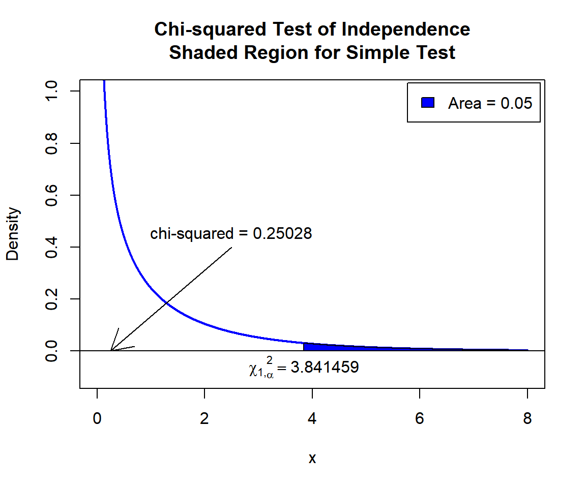
Chi-squared Test of Independence Shaded Region for Simple Test in R
See line charts, shading areas under a curve, lines & arrows on plots, mathematical expressions on plots, and legends on plots for more details on making the plot above.
3 Chi-squared Contingency Table Test Critical Value in R
To get the critical value for a chi-squared test in R, you can use
the qchisq() function for chi-squared distribution to
derive the quantile associated with the given level of significance
value \(\alpha\).
The critical value is qchisq(\(1-\alpha\), df).
Example:
For \(\alpha = 0.1\), and \(\text{df} = 2\).
[1] 4.605174 Chi-squared Test of Homogeneity (3x4 Table) in R
For test whether different age groups are homogeneous with regards to coffee preference.
| Age \ Coffee | Black | Latte | Irish | Mocha | Total |
|---|---|---|---|---|---|
| 18 to 25 | 12 | 44 | 67 | 80 | 203 |
| 26 to 45 | 18 | 64 | 97 | 117 | 296 |
| Above 45 | 15 | 19 | 27 | 33 | 94 |
| Total | 45 | 127 | 191 | 230 | 593 |
For the following null hypothesis \(H_0\), and alternative hypothesis \(H_1\), with the level of significance \(\alpha=0.1\).
\(H_0:\) the populations (age groups) are homogeneous.
\(H_1:\) the populations (age groups) are not homogeneous.
    Pearson's Chi-squared test

data:  rbind(c(12, 44, 67, 80), c(18, 64, 97, 117), c(15, 19, 27, 33))
X-squared = 11.204, df = 6, p-value = 0.08227
Interpretation:
P-value: With the p-value (\(p = 0.08227\)) being less than the level of significance 0.1, we reject the null hypothesis that the populations (age groups) are homogeneous. Hence, there are preferences based on age.
\(\chi^2_6\) T-statistic: With test statistics value (\(\chi^2_6 = 11.204\)) being in the critical region (shaded area), that is, \(\chi^2_6 = 11.204\) greater than \(\chi^2_{6, \alpha}=\text{qchisq(0.9, 6)}=10.6446407\), we reject the null hypothesis that the populations (age groups) are homogeneous. Hence, there are preferences based on age.
x = seq(0.01, 25, 1/1000); y = dchisq(x, df=6)
plot(x, y, type = "l",
     xlim = c(0, 25), ylim = c(-0.01, min(max(y), 1)),
     main = "Chi-squared Test of Homogeneity
Shaded Region",
     xlab = "x", ylab = "Density",
     lwd = 2, col = "blue")
abline(h=0)
# Add shaded region and legend
point = qchisq(0.9, 6)
polygon(x = c(x[x >= point], 25, point),
        y = c(y[x >= point], 0, 0),
        col = "blue")
legend("topright", c("Area = 0.1"),
       fill = c("blue"), inset = 0.01)
# Add critical value and chi-value
arrows(15, 0.05, 11.204, 0)
text(15, 0.055, "chi-squared = 11.204")
text(10.64464, -0.006, expression(chi[6][','][alpha]^2==10.64464))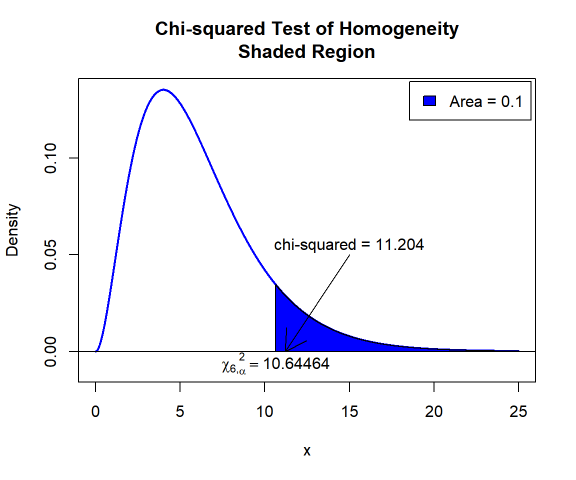
Chi-squared Test of Homogeneity Shaded Region for in R
5 Chi-squared Test of Independence (3x3 Table) in R
For test whether height and sleep hours are independent among 62 students.
| Height \ Hours | 9+ | 6 to 8 | <6 | Total |
|---|---|---|---|---|
| Tall | 7 | 6 | 8 | 21 |
| Medium | 6 | 8 | 7 | 21 |
| Short | 4 | 10 | 6 | 20 |
| Total | 17 | 24 | 21 | 62 |
For the following null hypothesis \(H_0\), and alternative hypothesis \(H_1\), with the level of significance \(\alpha=0.1\).
\(H_0:\) the row (height) and column (sleep hours) variables are independent.
\(H_1:\) the row (height) and column (sleep hours) variables are dependent.
    Pearson's Chi-squared test

data:  rbind(c(7, 6, 8), c(6, 8, 7), c(4, 10, 6))
X-squared = 2.0987, df = 4, p-value = 0.7176
Interpretation:
P-value: With the p-value (\(p = 0.7176\)) being greater than the level of significance 0.1, we fail to reject the null hypothesis that the row (height) and column (sleep hours) variables are independent. Hence, height does not impact sleep hours.
\(\chi^2_4\) T-statistic: With test statistics value (\(\chi^2_4 = 2.0987\)) being less than the critical value, \(\chi^2_{4,\alpha}=\text{qchisq(0.9, 4)}=7.7794403\) (or not in the shaded region), we fail to reject the null hypothesis that the row (height) and column (sleep hours) variables are independent. Hence, height does not impact sleep hours.
x = seq(0.01, 15, 1/1000); y = dchisq(x, df=4)
plot(x, y, type = "l",
     xlim = c(0, 15), ylim = c(-0.01, min(max(y), 1)),
     main = "Chi-squared Test of Independence
Shaded Region",
     xlab = "x", ylab = "Density",
     lwd = 2, col = "blue")
abline(h=0)
# Add shaded region and legend
point = qchisq(0.9, 4)
polygon(x = c(x[x >= point], 15, point),
        y = c(y[x >= point], 0, 0),
        col = "blue")
legend("topright", c("Area = 0.1"),
       fill = c("blue"), inset = 0.01)
# Add critical value and chi-value
arrows(3.5, 0.05, 2.0987, 0)
text(3.5, 0.055, "chi-squared = 2.0987")
text(7.77944, -0.008, expression(chi[4][','][alpha]^2==7.77944))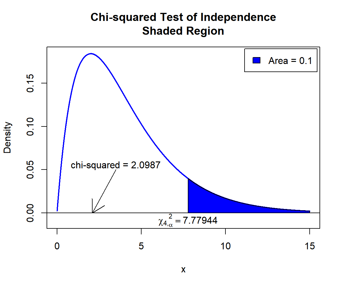
Chi-squared Test of Independence Shaded Region for in R
6 Chi-squared Contingency Table Test: Test Statistics, P-value & Degree of Freedom in R
Here for a chi-squared contingency table test, we show how to get the
test statistics (or chi-squared value), p-values, expected values, and
degrees of freedom from the chisq.test() function in R, or
by written code.
male = c(yes = 45, no = 55)
female = c(yes = 60, no = 65)
chsq_object = chisq.test(rbind(male, female),
                         correct = TRUE)
chsq_object
    Pearson's Chi-squared test with Yates' continuity correction

data:  rbind(male, female)
X-squared = 0.098437, df = 1, p-value = 0.7537
To get the test statistic or chi-squared value; observed and expected values:
\[\chi^2=\sum_{ij}\frac{(O_{ij}-E_{ij})^2}{E_{ij}},\]
Applicable to 2x2 tables only, for Yates’ continuity correction:
\[\chi^2=\sum_{ij}\frac{(|O_{ij}-E_{ij}|-c)^2}{E_{ij}}.\]
\(c = \min\{0.5, |O_{ij}-E_{ij}|\}\). \(|O_{ij}-E_{ij}|\) is equal for all \(ij\).
X-squared
0.0984375 [1] 0.0984375 yes no
male 45 55
female 60 65 yes no
male 46.66667 53.33333
female 58.33333 66.66667Same as (with continuity correction):
male = c(yes = 45, no = 55)
female = c(yes = 60, no = 65)
obs = rbind(male, female)
n = sum(obs)
rsum = rowSums(obs)
csum = colSums(obs)
exp = outer(rsum, csum, "*")/n
c = min(0.5, abs(obs-exp))
chi = sum(((abs(obs-exp)-c)^2)/exp)
chi
[1] 0.0984375 yes no
male 45 55
female 60 65 yes no
male 46.66667 53.33333
female 58.33333 66.66667Without continuity correction:
male = c(yes = 45, no = 55)
female = c(yes = 60, no = 65)
obs = rbind(male, female)
n = sum(obs)
rsum = rowSums(obs)
csum = colSums(obs)
exp = outer(rsum, csum, "*")/n
chi = sum(((obs-exp)^2)/exp)
chi
obs
exp
To get the p-value:
The p-value is, \(P \left(\chi^2_{df}> \text{observed} \right)\)
[1] 0.7537128Same as:
Note that the p-value depends on the \(\text{test statistics}\) (\(\chi^2_1 = 0.0984375\)), \(\text{degrees of freedom}\) (1). We also
use the distribution function pchisq() for the chi-squared
distribution in R.
[1] 0.7537128To get the degrees of freedom:
The degree of freedom is \((r-1)(c-1)\).
df
1 [1] 1Same as:
[1] 1The feedback form is a Google form but it does not collect any personal information.
Please click on the link below to go to the Google form.
Thank You!
Go to Feedback Form
Copyright © 2020 - 2026. All Rights Reserved by Stats Codes