Chi-squared Goodness of Fit Tests in R
- 1 Test Statistic for Chi-squared Goodness of Fit Test in R
- 2 Simple Chi-squared Goodness of Fit Test in R
- 3 Chi-squared Goodness of Fit Test Critical Value in R
- 4 Chi-squared Goodness of Fit Test for Weights in R
- 5 Chi-squared Goodness of Fit Test for Proportions in R
- 6 Chi-squared Goodness of Fit Test: Test Statistics, P-value & Degree of Freedom in R
Here, we discuss the chi-squared goodness of fit tests in R with interpretations, including, chi-squared value, expected values, p-values and critical values.
The chi-squared goodness of fit test in R can be performed with the
chisq.test() function from the base "stats" package.
The chi-squared goodness of fit test can be used to test whether an observed frequency distribution with \(k\) categories (cells) fits a proposed distribution as stated in the null hypothesis.
In the chi-squared goodness of fit test, the test statistic follows a chi-squared distribution with \(k − 1\) degrees of freedom when the null hypothesis is true.
| Question | Does the observed frequency distribution fit the proposed distribution? |
|---|---|
| Null Hypothesis, \(H_0\) | The proportion or count in each category fits that in the proposed distribution. |
| Alternate Hypothesis, \(H_1\) | The proportion or count in at least one category does not fit that in the proposed distribution. |
Sample Steps to Run a Chi-squared Goodness of Fit Test:
| Category | A | B | C | D | Total |
|---|---|---|---|---|---|
|
Observed Frequency |
37 | 32 | 19 | 12 | 100 |
|
Expected Frequency |
40 | 30 | 20 | 10 | 100 |
|
Expected Proportion |
0.40 | 0.30 | 0.20 | 0.10 | 1 |
# Run the chi-squared goodness of fit test with specifications
# Using the expected frequencies

chisq.test(c(37, 32, 19, 12),
           p = c(40, 30, 20, 10),
           rescale.p = TRUE)
    Chi-squared test for given probabilities

data:  c(37, 32, 19, 12)
X-squared = 0.80833, df = 3, p-value = 0.8475
Or:
# Run the chi-squared goodness of fit test with specifications
# Using the expected proportions

chisq.test(c(37, 32, 19, 12),
           p = c(0.4, 0.3, 0.2, 0.1))
    Chi-squared test for given probabilities

data:  c(37, 32, 19, 12)
X-squared = 0.80833, df = 3, p-value = 0.8475| Argument | Usage |
| x | Vector of values |
| p | A vector of probabilities or weights with the same length as x |
| rescale.p | Set to TRUE if p above is vector of weights, not
probabilities that sum to 1 |
Creating a Chi-squared Goodness of Fit Test Object:
# Create object
chsq_object = chisq.test(c(37, 32, 19, 12),
                         p = c(0.4, 0.3, 0.2, 0.1))

# Extract a component
chsq_object$statistic
X-squared
0.8083333 | Test Component | Usage |
| chsq_object$statistic | Test-statistic value |
| chsq_object$p.value | P-value |
| chsq_object$parameter | Degrees of freedom |
| chsq_object$observed | Observed counts |
| chsq_object$expected | Expected counts |
| chsq_object$residuals | Residual as (Obs. - Exp.)/sqrt(Exp.) |
1 Test Statistic for Chi-squared Goodness of Fit Test in R
The chi-squared goodness of fit test has test statistics that takes the form:
\[\chi^2=\sum_{i}\frac{(O_{i}-E_{i})^2}{E_{i}}.\]
With \(k\) categories, when the null hypothesis is true, \(\chi^2\) follows a chi-squared distribution (\(\chi^2_{k-1}\)) with degrees of freedom, \(k-1\),
\(O_i\) is the observed frequency in category (or cell) \(i\),
\(E_i\) is the expected frequency in category (or cell) \(i\), or \(E_i = np_i\),
where \(p_i\) is the distribution proportion in category (or cell) \(i\) and,
\(n\) is the total number of observations in all categories (or cells).
See also chi-squared contigency table tests.
2 Simple Chi-squared Goodness of Fit Test in R
Using an observed distribution for 187 randomly sampled sales, test the claim that there are the same amounts of sales in each weekday.
| Day | Mon | Tue | Wed | Thur | Fri | Total |
|---|---|---|---|---|---|---|
|
Observed Frequency |
34 | 42 | 33 | 37 | 41 | 187 |
|
Expected Proportion |
1/5 | 1/5 | 1/5 | 1/5 | 1/5 | 1 |
For the following null hypothesis \(H_0\), and alternative hypothesis \(H_1\), with the level of significance \(\alpha=0.05\).
\(H_0:\) the counts in each cell are equal.
\(H_1:\) the counts in at least one cell is different from the others.
For goodness of test, the chisq.test() function has
the default proportions as equal, hence, you do not
need to specify the "p" argument in this case.
Or:
    Chi-squared test for given probabilities

data:  c(34, 42, 33, 37, 41)
X-squared = 1.7433, df = 4, p-value = 0.7828
The test statistic, \(\chi^2_4\), is 1.7433,
the degree of freedom is \(k-1=4\),
the p-value, \(p\), is 0.7828.
Interpretation:
P-value: With the p-value (\(p = 0.7828\)) being greater than the level of significance 0.05, we fail to reject the null hypothesis that the counts in each cell are equal.
\(\chi^2_4\) T-statistic: With test statistics value (\(\chi^2_4 = 1.7433\)) being less than the critical value, \(\chi^2_{4,\alpha}=\text{qchisq(0.95, 4)}=9.487729\) (or not in the shaded region), we fail to reject the null hypothesis that the counts in each cell are equal.
x = seq(0.01, 18, 1/1000); y = dchisq(x, df=4)
plot(x, y, type = "l",
     xlim = c(0, 18), ylim = c(-0.02, min(max(y), 1)),
     main = "Chi-squared Test Goodnes of Fit Test
Shaded Region for Simple Test",
     xlab = "x", ylab = "Density",
     lwd = 2, col = "blue")
abline(h=0)
# Add shaded region and legend
point = qchisq(0.95, 4)
polygon(x = c(x[x >= point], 18, point),
        y = c(y[x >= point], 0, 0),
        col = "blue")
legend("topright", c("Area = 0.05"),
       fill = c("blue"), inset = 0.01)
# Add critical value and chi-value
arrows(10, 0.1, 1.7433, 0)
text(10, 0.11, "chi-squared = 1.7433")
text(9.487729, -0.01, expression(chi[4][','][alpha]^2==9.487729))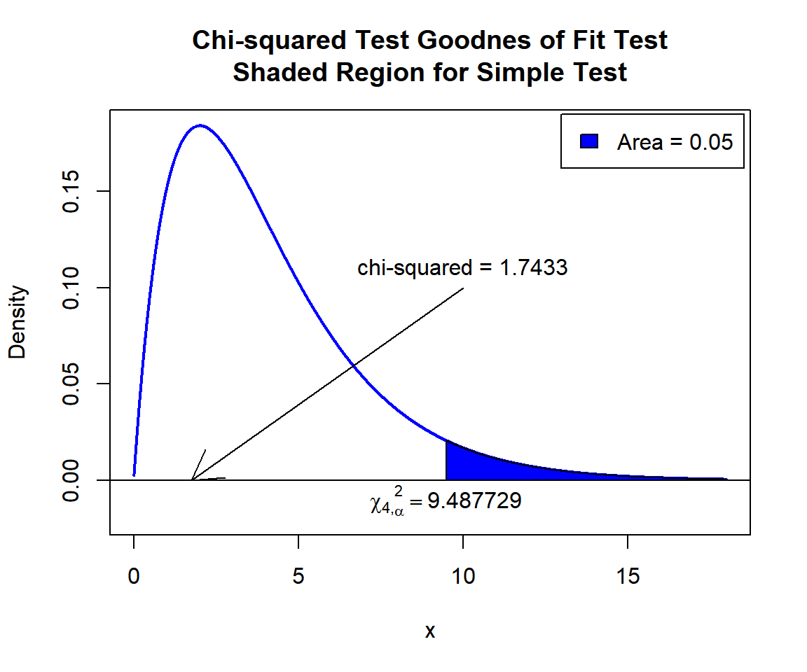
Chi-squared Test Goodness of Fit Test Shaded Region for Simple Test in R
See line charts, shading areas under a curve, lines & arrows on plots, mathematical expressions on plots, and legends on plots for more details on making the plot above.
3 Chi-squared Goodness of Fit Test Critical Value in R
To get the critical value for a chi-squared goodness of fit test in
R, you can use the qchisq() function for chi-squared
distribution to derive the quantile associated with the given level of
significance value \(\alpha\).
The critical value is qchisq(\(1-\alpha\), df).
Example:
For \(\alpha = 0.05\), and \(\text{df} = 5\).
[1] 11.07054 Chi-squared Goodness of Fit Test for Weights in R
Using an observed distribution for 534 randomly sampled students, test whether the proportion of the total students in the senior classes (Sen) doubles that of the total students in the junior classes (Jun), while the proportions are equal among the senior classes and equal among the junior classes.
| Class | Jun 1 | Jun 2 | Jun 3 | Sen 1 | Sen 2 | Sen 3 | Total |
|---|---|---|---|---|---|---|---|
|
Observed Frequency |
61 | 75 | 52 | 102 | 109 | 135 | 534 |
|
Expected (or Proposed) Weight |
1 | 1 | 1 | 2 | 2 | 2 | 9 |
For the following null hypothesis \(H_0\), and alternative hypothesis \(H_1\), with the level of significance \(\alpha=0.1\).
\(H_0:\) the proportion in each category fits that in the proposed distribution.
\(H_1:\) the proportion in each category does not fit that in the proposed distribution.
    Chi-squared test for given probabilities

data:  c(61, 75, 52, 102, 109, 135)
X-squared = 10.466, df = 5, p-value = 0.06305
Interpretation:
P-value: With the p-value (\(p = 0.06305\)) being less than the level of significance 0.1, we reject the null hypothesis that the proportion in each category fits that in the proposed distribution.
\(\chi^2_5\) T-statistic: With test statistics value (\(\chi^2_5 = 10.466\)) being in the critical region (shaded area), that is, \(\chi^2_5 = 10.466\) greater than \(\chi^2_{5, \alpha}=\text{qchisq(0.9, 5)}=9.2363569\), we reject the null hypothesis that the proportion in each category fits that in the proposed distribution.
x = seq(0.01, 25, 1/1000); y = dchisq(x, df=6)
plot(x, y, type = "l",
     xlim = c(0, 25), ylim = c(-0.01, min(max(y), 1)),
     main = "Chi-squared Goodness of Fit Test for Weights
Shaded Region",
     xlab = "x", ylab = "Density",
     lwd = 2, col = "blue")
abline(h=0)
# Add shaded region and legend
point = qchisq(0.9, 5)
polygon(x = c(x[x >= point], 25, point),
        y = c(y[x >= point], 0, 0),
        col = "blue")
legend("topright", c("Area = 0.1"),
       fill = c("blue"), inset = 0.01)
# Add critical value and chi-value
arrows(15, 0.05, 10.466, 0)
text(15, 0.055, "chi-squared = 10.466")
text(9.236357, -0.006, expression(chi[5][','][alpha]^2==9.236357))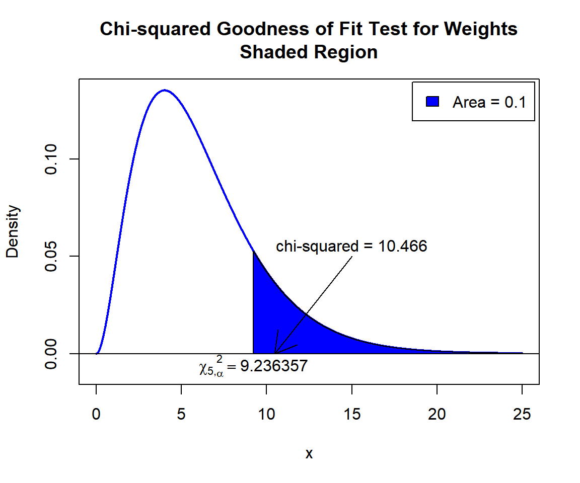
Chi-squared Goodness of Fit Test for Weights Shaded Region for in R
5 Chi-squared Goodness of Fit Test for Proportions in R
Using an observed distribution for 226 randomly sampled students in a club, test whether the proportions of participating students by year equal the proposed or expected proportions.
| Class | Year 1 | Year 3 | Year 3 | Year 4 | Total |
|---|---|---|---|---|---|
|
Observed Frequency |
88 | 65 | 55 | 44 | 226 |
|
Expected (or Proposed) Proportion |
4/10 | 3/10 | 2/10 | 1/10 | 1 |
For the following null hypothesis \(H_0\), and alternative hypothesis \(H_1\), with the level of significance \(\alpha=0.1\).
\(H_0:\) the proportion in each category fits that in the proposed distribution.
\(H_1:\) the proportion in each category does not fit that in the proposed distribution.
    Chi-squared test for given probabilities

data:  c(88, 65, 55, 18)
X-squared = 3.2404, df = 3, p-value = 0.356
Interpretation:
P-value: With the p-value (\(p = 0.356\)) being greater than the level of significance 0.1, we fail to reject the null hypothesis that the proportion in each category fits that in the proposed distribution.
\(\chi^2_3\) T-statistic: With test statistics value (\(\chi^2_3 = 3.2404\)) being less than the critical value, \(\chi^2_{3,\alpha}=\text{qchisq(0.9, 3)}=6.2513886\) (or not in the shaded region), we fail to reject the null hypothesis that the proportion in each category fits that in the proposed distribution.
x = seq(0, 15, 1/1000); y = dchisq(x, df=3)
plot(x, y, type = "l",
     xlim = c(0, 15), ylim = c(-0.015, min(max(y), 1)),
     main = "Chi-squared Goodness of Fit Test for Proportions
Shaded Region",
     xlab = "x", ylab = "Density",
     lwd = 2, col = "blue")
abline(h=0)
# Add shaded region and legend
point = qchisq(0.9, 3)
polygon(x = c(x[x >= point], 15, point),
        y = c(y[x >= point], 0, 0),
        col = "blue")
legend("topright", c("Area = 0.1"),
       fill = c("blue"), inset = 0.01)
# Add critical value and chi-value
arrows(7.5, 0.15, 3.2404, 0)
text(7.5, 0.16, "chi-squared = 3.2404")
text(6.251389, -0.01, expression(chi[3][','][alpha]^2==6.251389))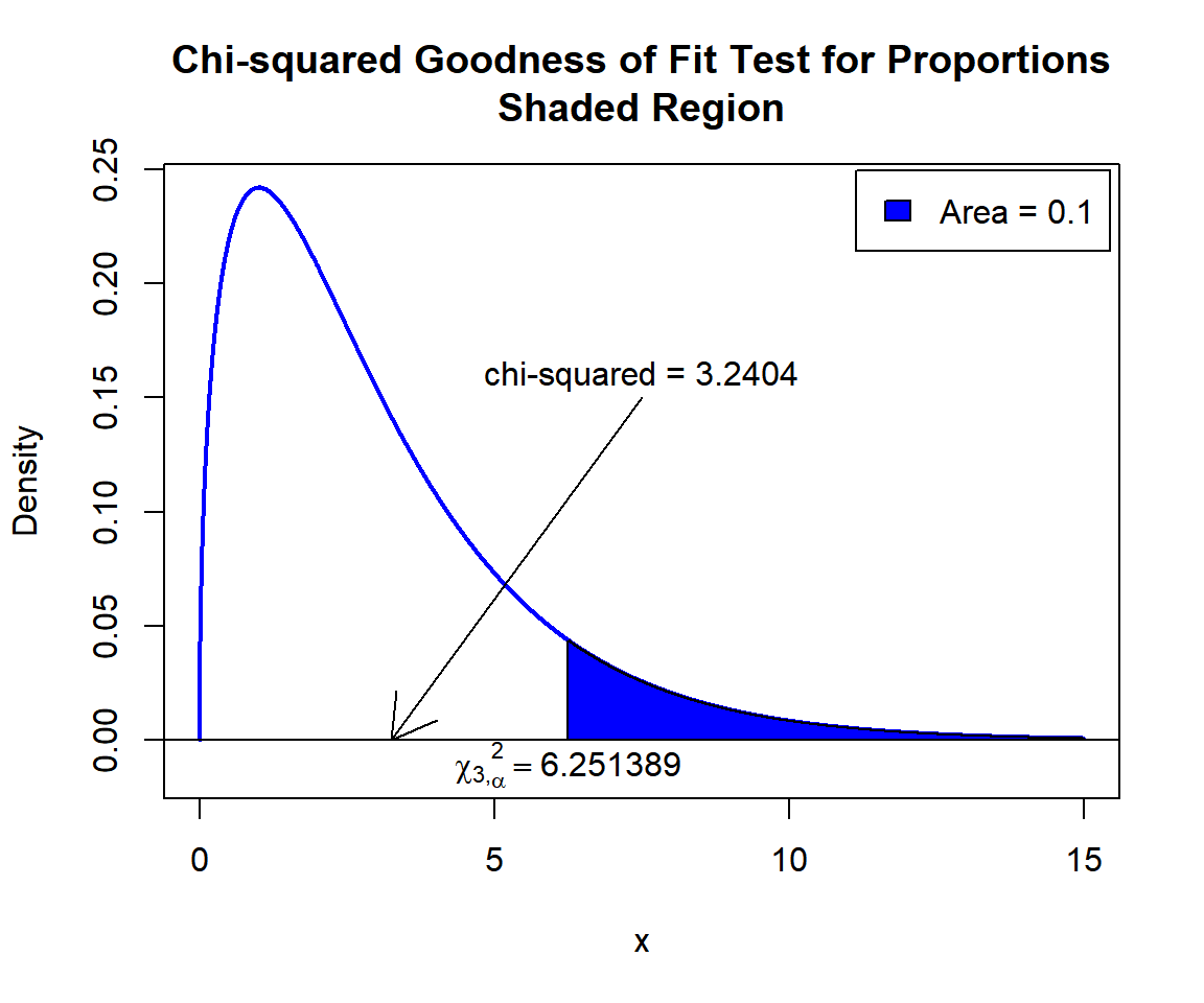
Chi-squared Goodness of Fit Test for Proportions Shaded Region for in R
6 Chi-squared Goodness of Fit Test: Test Statistics, P-value & Degree of Freedom in R
Here for a chi-squared goodness of fit test, we show how to get the
test statistics (or chi-squared value), p-values, expected values, and
degrees of freedom from the chisq.test() function in R, or
by written code.
    Chi-squared test for given probabilities

data:  c(32, 35, 28, 31)
X-squared = 16.357, df = 3, p-value = 0.000958
To get the test statistic or chi-squared value; observed and expected values:
\[\chi^2=\sum_{i}\frac{(O_i-E_i)^2}{E_i},\]
X-squared
16.35714 [1] 16.35714[1] 32 35 28 31[1] 21 42 42 21Same as:
obs = c(32, 35, 28, 31)
p = c(1/6, 2/6, 2/6, 1/6)
n = sum(obs)
exp = n*p
chi = sum(((obs-exp)^2)/exp)
chi
[1] 16.35714[1] 32 35 28 31[1] 21 42 42 21To get the p-value:
The p-value is, \(P \left(\chi^2_{df}> \text{observed} \right)\)
[1] 0.0009579516Same as:
Note that the p-value depends on the \(\text{test statistics}\) (\(\chi^2_3 = 16.35714\)), \(\text{degrees of freedom}\) (3). We also
use the distribution function pchisq() for the chi-squared
distribution in R.
[1] 0.0009579529To get the degrees of freedom:
The degree of freedom is \(k-1\).
df
3 [1] 3Same as:
[1] 3The feedback form is a Google form but it does not collect any personal information.
Please click on the link below to go to the Google form.
Thank You!
Go to Feedback Form
Copyright © 2020 - 2026. All Rights Reserved by Stats Codes