1 Test Statistic for Two-way ANOVA Test in R
2 Simple Two-way ANOVA Test in R
3 Two-way ANOVA Test Critical Value in R
4 Two-way ANOVA Test with Interaction Effect in R
5 Two-way ANOVA Test for Non-Orthogonal Design in R
6 Two-way ANOVA Test: Test Statistics, P-value & Degrees of Freedom in R
7 Two-way ANOVA Test with Interaction Effect: Test Statistics in R

Here, we discuss the two-way analysis of variance (ANOVA) test in R with interpretations, including, f-value, sum of squares, mean squares, p-values, and critical values.

The two-way ANOVA test in R can be performed with the anova() function from the base "stats" package.

The two-way ANOVA test can be used to test whether or not:

there is an effect from factor A (or row factor).
there is an effect from factor B (or column factor).
there is an effect from an interaction between the two factors.

In the two-way ANOVA test, the test statistic follows an F-distribution when the null hypothesis is true.

Two-way ANOVA Tests & Hypotheses for an Orthogonal or a Balanced Design
Question	Is there an effect from Factor A?	Is there an effect from Factor B?	Is there an effect from Factor A and Factor B interactions?
Null Hypothesis, \(H_0\)	\(\mu_{1\cdot} = \mu_{2\cdot} = \dots = \mu_{r\cdot}\)	\(\mu_{\cdot1} = \mu_{\cdot2} = \dots = \mu_{\cdot c}\)	\(\mu_{ij}-\mu_{i\cdot}-\mu_{\cdot j}\), for each cell \(ij\) are equal
Alternate Hypothesis, \(H_1\)	At least one group’s mean is different, hence, an effect	At least one group’s mean is different, hence, an effect	At least one interaction’s net mean is different, hence, an effect

Two-way ANOVA Tests & Hypotheses Non-Orthogonal Design
Question	Is there an effect from Factor A?	Is there an effect from Factor B after accounting for Factor A?	Is there an interaction effect after accounting for Factor A and/or Factor B effects?
Null Hypothesis, \(H_0\)	\(\mu_{1\cdot} = \mu_{2\cdot} = \dots = \mu_{r\cdot}\)	\(\mu_{\cdot1} = \mu_{\cdot2} = \dots = \mu_{\cdot c}\)	\(\mu_{ij}-\mu_{i\cdot}-\mu_{\cdot j}\), for each cell \(ij\) are equal
Alternate Hypothesis, \(H_1\)	At least one group’s mean is different, hence, an effect	At least one group’s mean is different, hence, an effect	At least one interaction’s net mean is different, hence, an effect

Sample Steps to Run a Two-way ANOVA Test:

# Create the factor data for the two-way ANOVA test
# Each row contains values for one group from factorA
# Each row contains 3 values for each group from factorB

y = c(5.1, 3.2, 5.1, 7.3, 2.7, 7.1,
      2.1, 4.9, 4.9, 6.8, 7.1, 5.0,
      8.4, 8.3, 6.8, 5.4, 5.0, 5.2)
factorA = c(rep("A1", 6),
            rep("A2", 6),
            rep("A3", 6))
factorB = c(rep("B1", 3), rep("B2", 3),
            rep("B1", 3), rep("B2", 3),
            rep("B1", 3), rep("B2", 3))
data.frame(y, factorA, factorB)


# Run the two-way ANOVA test with specifications

anova(lm(y ~ factorA + factorB))

Analysis of Variance Table

Response: y
          Df Sum Sq Mean Sq F value Pr(>F)
factorA    2  7.941  3.9706  1.2128 0.3268
factorB    1  0.436  0.4356  0.1330 0.7208
Residuals 14 45.834  3.2739

# For interaction effect
anova(lm(y ~ factorA + factorB + factorA:factorB))

Analysis of Variance Table

Response: y
                Df  Sum Sq Mean Sq F value Pr(>F)  
factorA          2  7.9411  3.9706  1.8744 0.1957  
factorB          1  0.4356  0.4356  0.2056 0.6583  
factorA:factorB  2 20.4144 10.2072  4.8185 0.0291 *
Residuals       12 25.4200  2.1183                 
---
Signif. codes:  0 '***' 0.001 '**' 0.01 '*' 0.05 '.' 0.1 ' ' 1

Table of Some Two-way ANOVA Tests Arguments in R
Argument	Usage
lm(y ~ x + w)	y contains the sample values, x and w are factors and specify the groups they belong
lm(y ~ x + w + x:w)	y contains the sample values, x and w are factors and specify the groups they belong, x:w for interaction
lm(y ~ x + x:w)	y contains the sample values, x and w are factors and specify the groups they belong, x:w for interaction

Creating a Two-way ANOVA Test Object:

# Create data
y = rnorm(240, 50, 2)
factorA = rep(c("A1", "A2", "A3", "A4"),
              each = 60)
factorB = rep(c("B1", "B2", "B3"),
              each = 20, times = 4)
#data.frame(y, factorA, factorB)

# Create object
aov_object = anova(lm(y ~ factorA + factorB))

# Extract a component
aov_object$`F value`[1:2]

[1] 0.50137487 0.05430339

# For interaction effect

# Create object
aov_object = anova(lm(y ~ factorA + factorB + factorA:factorB))

# Extract a component
aov_object$`F value`[1:3]

[1] 0.49673427 0.05380077 0.63902548

Table of Some Two-way ANOVA Test Object Outputs in R
`anova()` Component	Usage
aov_object$`F value`[1:2]	Test-statistic value
aov_object$`Pr(>F)`[1:2]	P-value
aov_object$`F value`[1:3]	Test-statistic value with interaction effect
aov_object$`Pr(>F)`[1:3]	P-value with interaction effect
aov_object$Df	Degrees of freedom
aov_object$`Sum Sq`	Sum of squares
aov_object$`Mean Sq`	Mean squares

1 Test Statistic for Two-way ANOVA Test in R

The two-way analysis of variance test has test statistics, $F$, of the form:

Table of Two-way ANOVA Calculations
Source of Variation	Degrees of Freedom (DF)	Sums of Squares (SS)	Sums of Squares (SS) –ORTHOGONAL DESIGN ONLY–	Mean Square (MS)	F	P-value
Factor A	$r-1$	$SSA$	$\sum_{i=1}^r n_{i\cdot}(\bar y_{i\cdot}-\bar y_{\cdot \cdot})^2$	$\frac{SSA}{DFA}$	$\frac{MSA}{MSR}$	$P(F_{r-1 \;,\; n-r-c+1}>F)$
Factor B	$c-1$	$SSB$	$\sum_{j=1}^c n_{\cdot j}(\bar y_{\cdot j}-\bar y_{\cdot \cdot})^2$	$\frac{SSB}{DFB}$	$\frac{MSB}{MSR}$	$P(F_{c-1 \;,\; n-r-c+1}>F)$
Residuals	$n-r-c+1$	$SSR$	$\sum_{i=1}^r \sum_{j=1}^c \sum_{k=1}^{n_{ij}} (y_{ijk}-\bar y_{i\cdot}-\bar y_{\cdot j}+\bar y_{\cdot \cdot})^2$	$\frac{SSR}{DFR}$
Total	$n-1$	$SST$	$\sum_{i=1}^r \sum_{j=1}^c \sum_{k=1}^{n_{ij}} (y_{ijk}-\bar y_{\cdot \cdot})^2$

Table of Two-way ANOVA Calculations with Interaction Effects
Source of Variation	Degrees of Freedom (DF)	Sums of Squares (SS)	Sums of Squares (SS) –ORTHOGONAL DESIGN ONLY–	Mean Square (MS)	F	P-value
Factor A	$r-1$	$SSA$	$\sum_{i=1}^r n_{i\cdot}(\bar y_{i\cdot}-\bar y_{\cdot \cdot})^2$	$\frac{SSA}{DFA}$	$\frac{MSA}{MSR}$	$P(F_{r-1 \;,\; n−rc}>F)$
Factor B	$c-1$	$SSB$	$\sum_{j=1}^c n_{\cdot j}(\bar y_{\cdot j}-\bar y_{\cdot \cdot})^2$	$\frac{SSB}{DFB}$	$\frac{MSB}{MSR}$	$P(F_{c-1 \;,\; n−rc}>F)$
Interaction AB	$(r-1)(c-1)$	$SSAB$	$\sum_{i=1}^r \sum_{j=1}^c n_{ij}(\bar y_{ij}-\bar y_{i\cdot}-\bar y_{\cdot j}+\bar y_{\cdot \cdot})^2$	$\frac{SSAB}{DFAB}$	$\frac{MSAB}{MSR}$	$P(F_{(r-1)(c-1) \;,\; n−rc}>F)$
Residuals	$n-rc$	$SSR$	$\sum_{i=1}^r \sum_{j=1}^c \sum_{k=1}^{n_{ij}} (y_{ijk}-\bar y_{ij})^2$	$\frac{SSR}{DFR}$
Total	$n-1$	$SST$	$\sum_{i=1}^r \sum_{j=1}^c \sum_{k=1}^{n_{ij}} (y_{ijk}-\bar y_{\cdot \cdot})^2$

For independent random samples that come from normal distributions, $F$ is said to follow the F-distribution $\left(df1, df2\right)$ when the null hypothesis is true, with $df1$ numerator degrees of freedom, and $df2$ denominator degrees of freedom.

Orthogonal Design: In the two-way analysis of variance, an orthogonal design is one where $n_{ij}=\frac{n_{i\cdot}n_{\cdot j}}{n}$ for all row and column interactions (cells) $ij$. That is, each cell size equals row total, times column total, divided by total observation in experiment. Hence, the cell size proportions in each row are the same for all rows, and the cell size proportions in each column are the same for all columns.

In R, an important implication of orthogonal designs is that the order of the factors into the model does not matter, whereas it does for non-orthogonal designs.

In the balanced design, the number of observations for each factors interaction are equal, that is, $n_{ij}$ are equal for all row and column interactions (cells) $ij$. Hence, any balanced design is orthogonal.

Notations

See the notations table in the next tab.

$r$ is the total number of groups (rows) in Factor A,

$c$ is the total number of groups (columns) in Factor B,

$n_{ij}$ is the number of observations from row $i$ and column $j$ interaction,

$n_{i\cdot}$ is the number of observations in group (row) $i$ from Factor A,

$n_{\cdot j}$ is the number of observations in group (column) $j$ from Factor B,

$n$ is the total number of observations, $\sum_{i=1}^r \sum_{j=1}^c n_{ij}$,

$y_{ijk}$ is the $k$th observation from row $i$ and column $j$ interaction,

$\bar y_{ij}$ is the mean of observations from row $i$ and column $j$ interaction,

$\bar y_{i\cdot}$ is the mean of observations in group (row) $i$ from Factor A,

$\bar y_{\cdot j}$ is the mean of observations in group (column) $j$ from Factor B,

$\bar y_{\cdot \cdot}$ is the overall mean.

Notations Table

Notations of Cell Means and Number of Observations in Cells
	Factor B (Column Factor)
Factor A (Row Factor)		Column 1	Column 2	$\cdots$	Column $c$	Aggregate
	Row 1	$\bar y_{11}$ $n_{11}$	$\bar y_{12}$ $n_{12}$	$\cdots$	$\bar y_{1c}$ $n_{1c}$	$\bar y_{1\cdot}$ = Row Mean $n_{1\cdot}$ = Row Size
	Row 2	$\bar y_{21}$ $n_{21}$	$\bar y_{22}$ $n_{22}$	$\cdots$	$\bar y_{2c}$ $n_{2c}$	$\bar y_{2\cdot}$ = Row Mean $n_{2\cdot}$ = Row Size
	$\vdots$	$\vdots$	$\vdots$	$\ddots$	$\vdots$	$\vdots$
	Row $r$	$\bar y_{r1}$ $n_{r1}$	$\bar y_{r2}$ $n_{r2}$	$\cdots$	$\bar y_{rc}$ $n_{rc}$	$\bar y_{r\cdot}$ = Row Mean $n_{r\cdot}$ = Row Size
	Aggregate	$\bar y_{\cdot1}$ = Col Mean $n_{\cdot1}$ = Col Size	$\bar y_{\cdot2}$ = Col Mean $n_{\cdot2}$ = Col Size	$\cdots$	$\bar y_{\cdot c}$ = Col Mean $n_{\cdot c}$ = Col Size	$\bar y_{\cdot \cdot}$ = Grand Mean $n$ = Total Size

2 Simple Two-way ANOVA Test in R

Tabel of Cell Values
	Factor B (Column Factor)
Factor A (Row Factor)		B1	B2	Aggregate
	A1	18.8, 20.2, 17.9, 19.6	20.8, 23.3, 18.9, 18.7	$\bar y_{1\cdot} = 19.77500$, $n_{1\cdot} = 8$
	A2	20.6, 20.5, 22.5, 22.8	22.6, 22.8, 20.3, 22.6	$\bar y_{2\cdot} = 21.8375$, $n_{2\cdot} = 8$
	A3	21.2, 19.4, 18.2, 19.8	21.2, 17.1, 21.5, 21.0	$\bar y_{3\cdot} = 19.92500$, $n_{3\cdot} = 8$
	Aggregate	$\bar y_{\cdot1} = 20.1250$, $n_{\cdot1} = 12$	$\bar y_{\cdot2} = 20.9000$, $n_{\cdot2} = 12$	$\bar y_{\cdot \cdot} = 20.5125$, $n = 24$

Enter the data by hand.

y = c(18.8, 20.2, 17.9, 19.6, 20.8, 23.3, 18.9, 18.7,
      20.6, 20.5, 22.5, 22.8, 22.6, 22.8, 20.3, 22.6,
      21.2, 19.4, 18.2, 19.8, 21.2, 17.1, 21.5, 21.0)
factorA = c(rep("A1", 8),
            rep("A2", 8),
            rep("A3", 8))
factorB = c(rep("B1", 4), rep("B2", 4),
            rep("B1", 4), rep("B2", 4),
            rep("B1", 4), rep("B2", 4))

Check variability between and within groups with a boxplot.

The median lines appear to be on different levels especially by factor A, hence, there appears to be factor effects.

boxplot(y ~ factorA:factorB,
     main = "Y by Factors and Groups",
     xlab = "Groups",
     ylab = "Y Value")

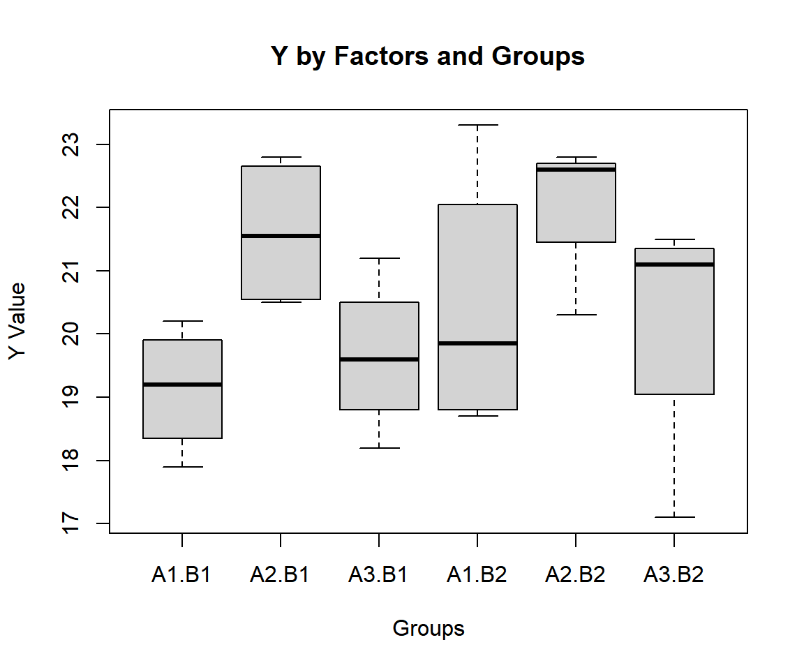
Simple Two-way ANOVA Test Box Plot in R

The group and overall means, variances and lengths are:

c(tapply(y, factorA, mean),
  tapply(y, factorB, mean), mean(y))

     A1      A2      A3      B1      B2         
19.7750 21.8375 19.9250 20.1250 20.9000 20.5125

c(tapply(y, factorA, var),
  tapply(y, factorB, var), var(y))

      A1       A2       A3       B1       B2          
2.867857 1.305536 2.590714 2.331136 3.569091 2.978533

c(tapply(y, factorA, length),
  tapply(y, factorB, length), length(y))

A1 A2 A3 B1 B2    
 8  8  8 12 12 24

For the following null hypothesis $H_0$, and alternative hypothesis $H_1$, with the level of significance $\alpha=0.05$.

Factor A	Factor B
$H_0:$ there is no effect from Factor A $(\mu_{1\cdot} = \mu_{2\cdot} = \mu_{3\cdot})$.	$H_0:$ there is no effect from Factor B $(\mu_{\cdot 1} = \mu_{\cdot 2})$.
$H_1:$ at least one group’s mean is different, hence, an effect.	$H_1:$ at least one group’s mean is different, hence, an effect.

Because this is an orthogonal design, the order of factor A and factor B in the model does not matter.

anova(lm(y ~ factorA + factorB))

Analysis of Variance Table

Response: y
          Df Sum Sq Mean Sq F value  Pr(>F)  
factorA    2 21.157 10.5787  4.8366 0.01935 *
factorB    1  3.604  3.6037  1.6476 0.21396  
Residuals 20 43.745  2.1872                  
---
Signif. codes:  0 '***' 0.001 '**' 0.01 '*' 0.05 '.' 0.1 ' ' 1

Factor A	Factor B
The test statistic, $F$, is 4.8366,	The test statistic, $F$, is 1.6476,
the degrees of freedom, are numerator df $r-1= 2$, denominator df $n-r-c+1= 20$,	the degrees of freedom, are numerator df $c-1= 1$, denominator df $n-r-c+1= 20$,
the p-value, $p$, is 0.01935.	the p-value, $p$, is 0.21396.

Interpretation:

Factor A	Factor B
P-value: With the p-value $(p = 0.01935)$ being less than the level of significance 0.05, we reject the null hypothesis that there is no effect from Factor A.	P-value: With the p-value $(p = 0.21396)$ being greater than the level of significance 0.05, we fail to reject the null hypothesis that there is no effect from Factor B.
$F$ T-statistic: With test statistics value $(F_{2, 20} = 4.8366)$ being in the critical region (shaded area), that is, $F_{2, 20} = 4.8366$ greater than $F_{2, 20, \alpha}=\text{qf(0.95, 2, 20)}$$=3.4928285$, we reject the null hypothesis that there is no effect from Factor A.	$F$ T-statistic: With test statistics value $(F_{1, 20} = 1.6476)$ being less than the critical value, $F_{1, 20, \alpha}=\text{qf(0.95, 1, 20)}$$=4.3512435$ (or not in the shaded region), we fail to reject the null hypothesis that there is no effect from Factor B.

par(mfrow=c(1,2))
#Plot Factor A
x = seq(0.01, 5, 1/1000); y = df(x, df1=2, df2=20)
plot(x, y, type = "l",
     xlim = c(0, 5), ylim = c(-0.06, min(max(y), 1)),
     main = "Two-way ANOVA Test (Factor A)
Shaded Region for Simple Test",
     xlab = "x", ylab = "Density",
     lwd = 2, col = "blue")
abline(h=0)
# Add shaded region and legend
point = qf(0.95, 2, 20)
polygon(x = c(x[x >= point], 5, point),
        y = c(y[x >= point], 0, 0),
        col = "blue")
legend("topright", c("Area = 0.05"),
       fill = c("blue"), inset = 0.01)
# Add critical value and F-value
arrows(2.5, 0.4, 4.8366, 0)
text(2.5, 0.45, "F = 4.8366")
text(3.492828, -0.04, expression(F[alpha]==3.492828))
#Plot Factor B
x = seq(0.01, 5, 1/1000); y = df(x, df1=1, df2=20)
plot(x, y, type = "l",
     xlim = c(0, 5), ylim = c(-0.06, min(max(y), 1)),
     main = "Two-way ANOVA Test (Factor B)
Shaded Region for Simple Test",
     xlab = "x", ylab = "Density",
     lwd = 2, col = "blue")
abline(h=0)
# Add shaded region and legend
point = qf(0.95, 1, 20)
polygon(x = c(x[x >= point], 5, point),
        y = c(y[x >= point], 0, 0),
        col = "blue")
legend("topright", c("Area = 0.05"),
       fill = c("blue"), inset = 0.01)
# Add critical value and F-value
arrows(2.5, 0.4, 1.6476, 0)
text(2.5, 0.45, "F = 1.6476")
text(4.351244, -0.04, expression(F[alpha]==4.351244))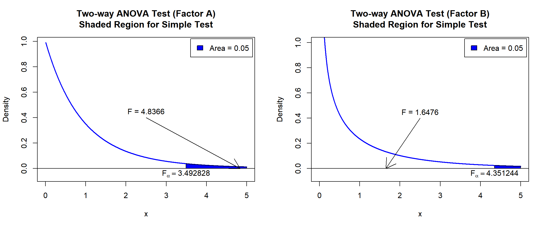

Two-way ANOVA Test Shaded Region for Simple Test in R

See line charts, shading areas under a curve, lines & arrows on plots, mathematical expressions on plots, and legends on plots for more details on making the plots above.

3 Two-way ANOVA Test Critical Value in R

To get the critical value for a two-way ANOVA test in R, you can use the qf() function for F-distribution to derive the quantile associated with the given level of significance value $\alpha$.

The critical values is qf($1-\alpha$, df1, df2).

Example:

For $\alpha = 0.05$, $\text{df1} = 2$, and $\text{df2} = 30$.

qf(0.95, 2, 30)

[1] 3.31583

4 Two-way ANOVA Test with Interaction Effect in R

Using the warpbreaks data from the "datasets" package with 10 sample rows from 54 rows below:

warpbreaks

   breaks wool tension
1      26    A       L
5      70    A       L
19     36    A       H
23     10    A       H
25     28    A       H
30     29    B       L
36     44    B       L
44     39    B       M
49     17    B       H
54     28    B       H

Check variability between and within groups with a boxplot.

boxplot(breaks ~ wool + tension, data = warpbreaks,
     main = "Y by Factor and Groups",
     xlab = "Groups",
     ylab = "Y Value")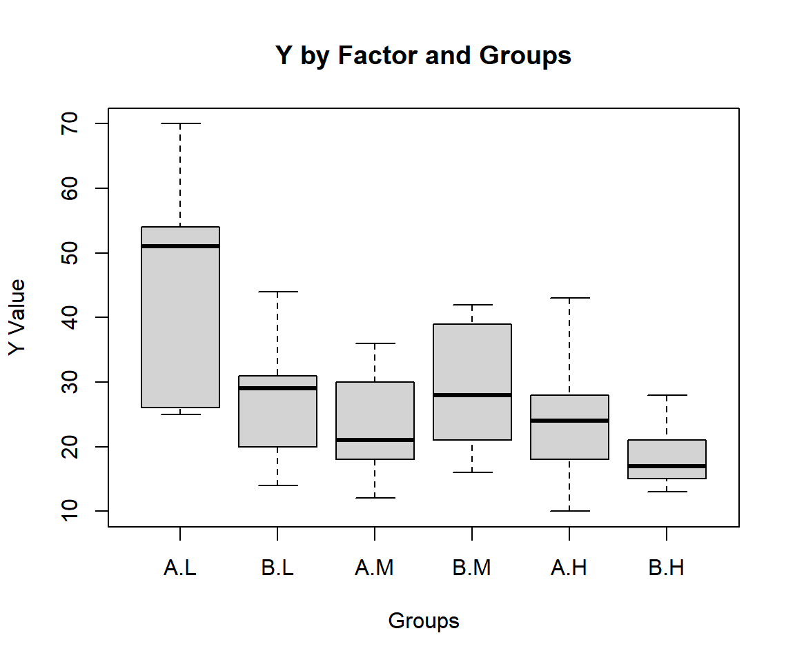

Two-way ANOVA Test Box Plot in R

For "wool" as Factor A and "tension" as Factor B.

The group, interaction and overall means, variances and lengths are:

y = warpbreaks$breaks; factorA = warpbreaks$wool;
factorB = warpbreaks$tension; intr = factorA:factorB
c(tapply(y, factorA, mean),
  tapply(y, factorB, mean),
  tapply(y, intr, mean), mean(y))

       A        B        L        M        H      A:L      A:M      A:H 
31.03704 25.25926 36.38889 26.38889 21.66667 44.55556 24.00000 24.55556 
     B:L      B:M      B:H          
28.22222 28.77778 18.77778 28.14815

c(tapply(y, factorA, var),
  tapply(y, factorB, var),
  tapply(y, intr, var), var(y))

        A         B         L         M         H       A:L       A:M       A:H 
251.26781  86.50712 270.48693  83.19281  69.76471 327.52778  75.00000 105.52778 
      B:L       B:M       B:H           
 97.19444  88.94444  23.94444 174.20405

c(tapply(y, factorA, length),
  tapply(y, factorB, length),
  tapply(y, intr, length), length(y))

  A   B   L   M   H A:L A:M A:H B:L B:M B:H     
 27  27  18  18  18   9   9   9   9   9   9  54

For the following null hypothesis $H_0$, and alternative hypothesis $H_1$, with the level of significance $\alpha=0.05$.

Factor A	Factor B	Interaction AB
$H_0:$ there is no effect from Factor A $(\mu_{1\cdot} = \mu_{2\cdot})$.	$H_0:$ there is no effect from Factor B $(\mu_{\cdot 1} = \mu_{\cdot 2} = \mu_{\cdot 3})$.	$H_0:$ there is no interaction effect $(\mu_{ij}-\mu_{i\cdot}-\mu_{\cdot j}$, for each cell $ij$ are all equal).
$H_1:$ at least one group’s mean is different, hence, an effect.	$H_1:$ at least one group’s mean is different, hence, an effect.	$H_1:$ at least one interaction’s net mean is different, hence, an effect.

Because this is an orthogonal design, the order of factor A and factor B in the model does not matter.

anova(lm(breaks ~ wool + tension + wool:tension,
         data = warpbreaks))

Or:

anova(lm(y ~ factorA + factorB + factorA:factorB))

Analysis of Variance Table

Response: y
                Df Sum Sq Mean Sq F value    Pr(>F)    
factorA          1  450.7  450.67  3.7653 0.0582130 .  
factorB          2 2034.3 1017.13  8.4980 0.0006926 ***
factorA:factorB  2 1002.8  501.39  4.1891 0.0210442 *  
Residuals       48 5745.1  119.69                      
---
Signif. codes:  0 '***' 0.001 '**' 0.01 '*' 0.05 '.' 0.1 ' ' 1

Interpretation:

Factor A	Factor B	Interaction AB
P-value: With the p-value $(p = 0.0582130)$ being greater than the level of significance 0.05, we fail to reject the null hypothesis that there is no effect from Factor A.	P-value: With the p-value $(p = 0.0006926)$ being less than the level of significance 0.05, we reject the null hypothesis that there is no effect from Factor B.	P-value: With the p-value $(p = 0.0210442)$ being less than the level of significance 0.05, we reject the null hypothesis that there is no interaction effect.
$F$ T-statistic: With test statistics value $(F_{1, 48} = 3.7653)$ being less than the critical value, $F_{1, 48, \alpha}=\text{qf(0.95, 1, 48)}$$=4.0426521$ (or not in the shaded region), we fail to reject the null hypothesis that there is no effect from Factor A.	$F$ T-statistic: With test statistics value $(F_{2, 48} = 8.4980)$ being in the critical region (shaded area), that is, $F_{2, 48} = 8.4980$ greater than $F_{2, 48, \alpha}=\text{qf(0.95, 2, 48)}$$=3.1907273$, we reject the null hypothesis that there is no effect from Factor B.	$F$ T-statistic: With test statistics value $(F_{2, 48} = 4.1891)$ being in the critical region (shaded area), that is, $F_{2, 48} = 4.1891$ greater than $F_{2, 48, \alpha}=\text{qf(0.95, 2, 48)}$$=3.1907273$, we reject the null hypothesis that there is no interaction effect.

par(mfrow=c(2,2))
#Plot Factor A
x = seq(0.01, 5, 1/1000); y = df(x, df1=1, df2=48)
plot(x, y, type = "l",
     xlim = c(0, 5), ylim = c(-0.06, min(max(y), 1)),
     main = "Two-way ANOVA Test (Factor A)
Shaded Region",
     xlab = "x", ylab = "Density",
     lwd = 2, col = "blue")
abline(h=0)
# Add shaded region and legend
point = qf(0.95, 1, 48)
polygon(x = c(x[x >= point], 5, point),
        y = c(y[x >= point], 0, 0),
        col = "blue")
legend("topright", c("Area = 0.05"),
       fill = c("blue"), inset = 0.01)
# Add critical value and F-value
arrows(2.5, 0.4, 3.7653, 0)
text(2.5, 0.45, "F = 3.7653")
text(4.042652, -0.04, expression(F[alpha]==4.042652))
#Plot Factor B
x = seq(0.01, 9, 1/1000); y = df(x, df1=2, df2=48)
plot(x, y, type = "l",
     xlim = c(0, 9), ylim = c(-0.06, min(max(y), 1)),
     main = "Two-way ANOVA Test (Factor B)
Shaded Region",
     xlab = "x", ylab = "Density",
     lwd = 2, col = "blue")
abline(h=0)
# Add shaded region and legend
point = qf(0.95, 2, 48)
polygon(x = c(x[x >= point], 9, point),
        y = c(y[x >= point], 0, 0),
        col = "blue")
legend("topright", c("Area = 0.05"),
       fill = c("blue"), inset = 0.01)
# Add critical value and F-value
arrows(2.5, 0.4, 8.4980, 0)
text(2.5, 0.45, "F = 8.4980")
text(3.190727, -0.04, expression(F[alpha]==3.190727))
#Plot Interaction A:B
x = seq(0.01, 5, 1/1000); y = df(x, df1=2, df2=48)
plot(x, y, type = "l",
     xlim = c(0, 5), ylim = c(-0.06, min(max(y), 1)),
     main = "Two-way ANOVA Test (Interaction A:B)
Shaded Region",
     xlab = "x", ylab = "Density",
     lwd = 2, col = "blue")
abline(h=0)
# Add shaded region and legend
point = qf(0.95, 2, 48)
polygon(x = c(x[x >= point], 5, point),
        y = c(y[x >= point], 0, 0),
        col = "blue")
legend("topright", c("Area = 0.05"),
       fill = c("blue"), inset = 0.01)
# Add critical value and F-value
arrows(2.5, 0.4, 4.1891, 0)
text(2.5, 0.45, "F = 4.1891")
text(3.190727, -0.04, expression(F[alpha]==3.190727))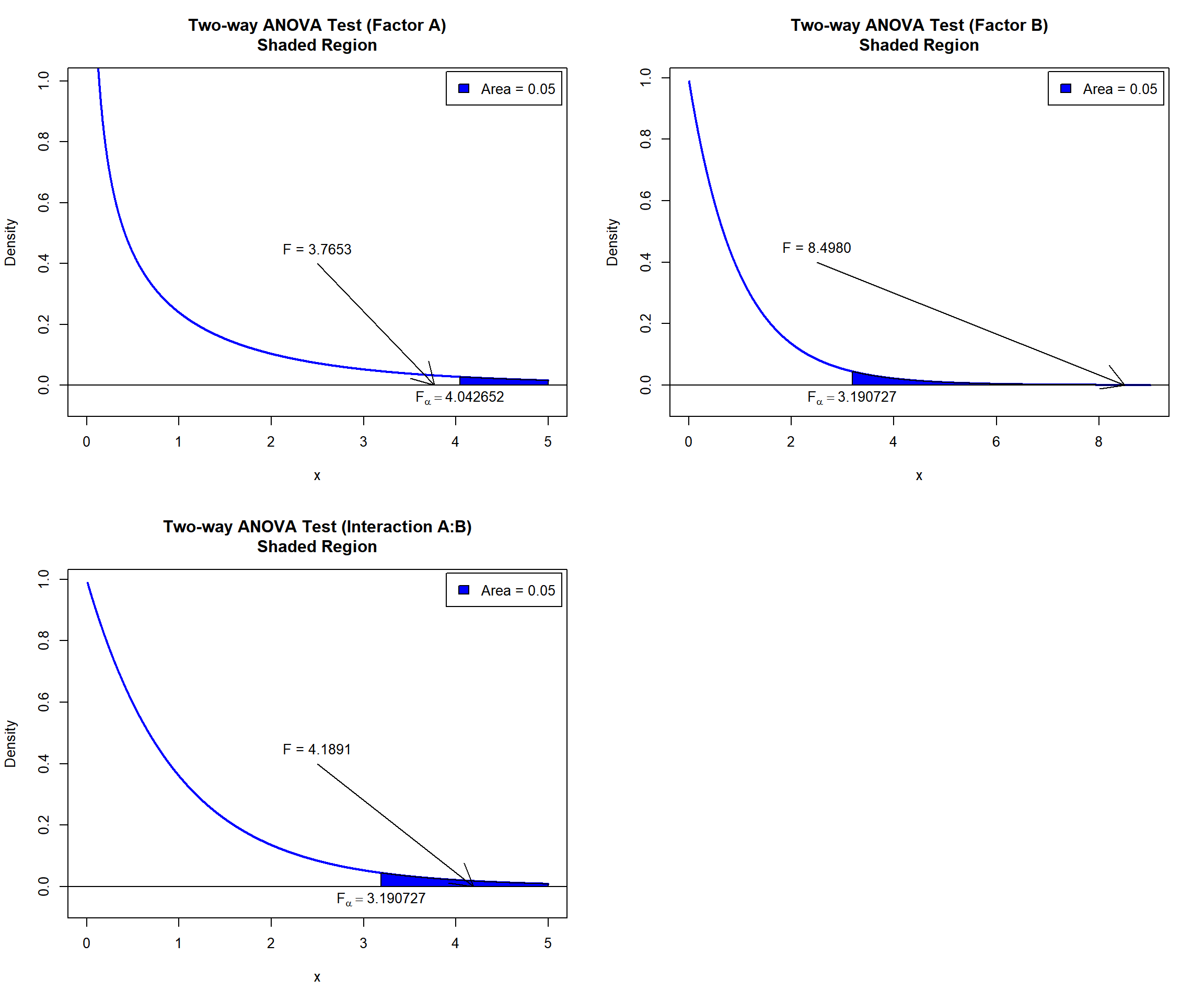

Two-way ANOVA Test Shaded Region in R

5 Two-way ANOVA Test for Non-Orthogonal Design in R

Using a subset of the warpbreaks data from the "datasets" package with 10 sample rows from 48 subset of rows below:

set.seed(1)
wpbk = warpbreaks[sample(1:54, 48, replace = FALSE),]
wpbk

   breaks wool tension
4      25    A       L
14     12    A       M
42     28    B       M
37     42    B       M
20     21    A       H
27     26    A       H
47     21    B       H
35     20    B       L
32     29    B       L
16     35    A       M

For "wool" as Factor A and "tension" as Factor B.

The group, interaction and overall means, variances and lengths are:

y = wpbk$breaks; factorA = wpbk$wool;
factorB = wpbk$tension; intr = factorA:factorB
c(tapply(y, factorA, mean),
  tapply(y, factorB, mean),
  tapply(y, intr, mean), mean(y))

       A        B        L        M        H      A:L      A:M      A:H 
30.43478 25.52000 34.41176 27.92857 21.29412 41.37500 24.66667 24.55556 
     B:L      B:M      B:H          
28.22222 30.37500 17.62500 27.87500

c(tapply(y, factorA, var),
  tapply(y, factorB, var),
  tapply(y, intr, var), var(y))

        A         B         L         M         H       A:L       A:M       A:H 
213.98419  89.76000 212.63235  87.91758  71.47059 270.26786 100.66667 105.52778 
      B:L       B:M       B:H           
 97.19444  75.41071  13.69643 152.15426

c(tapply(y, factorA, length),
  tapply(y, factorB, length),
  tapply(y, intr, length), length(y))

  A   B   L   M   H A:L A:M A:H B:L B:M B:H     
 23  25  17  14  17   8   6   9   9   8   8  48

For the following null hypothesis $H_0$, and alternative hypothesis $H_1$, with the level of significance $\alpha=0.1$.

Test 1	Test 2
$H_0:$ there is no effect from Factor A $(\mu_{1\cdot} = \mu_{2\cdot})$ accounting for factor A effects first.	$H_0:$ there is no effect from Factor A $(\mu_{1\cdot} = \mu_{2\cdot})$ accounting for Factor B effects first.
$H_1:$ at least one group’s mean is different accounting for factor A effects first, hence, an effect.	$H_1:$ at least one group’s mean is different accounting for Factor B effects first, hence, an effect.

Because this is a non-orthogonal design, the order of factor A and factor B in the model matters.

For test 1, "wool" should go into the model first.

anova(lm(breaks ~ wool + tension, 
         data = wpbk))

Or:

anova(lm(y ~ factorA + factorB))

Analysis of Variance Table

Response: y
          Df Sum Sq Mean Sq F value   Pr(>F)   
factorA    1  289.4  289.36  2.3895 0.129314   
factorB    2 1533.7  766.86  6.3328 0.003828 **
Residuals 44 5328.2  121.09                    
---
Signif. codes:  0 '***' 0.001 '**' 0.01 '*' 0.05 '.' 0.1 ' ' 1

For test 2, "wool" should go into the model second.

anova(lm(breaks ~ tension + wool,
         data = wpbk))

Or:

anova(lm(y ~ factorB + factorA))

Analysis of Variance Table

Response: y
          Df Sum Sq Mean Sq F value   Pr(>F)   
factorB    2 1462.7  731.34  6.0394 0.004813 **
factorA    1  360.4  360.41  2.9763 0.091511 . 
Residuals 44 5328.2  121.09                    
---
Signif. codes:  0 '***' 0.001 '**' 0.01 '*' 0.05 '.' 0.1 ' ' 1

Test 1	Test 2
P-value: With the p-value $(p = 0.129314)$ being greater than the level of significance 0.1, we fail to reject the null hypothesis that there is no effect from Factor A.	P-value: With the p-value $(p = 0.091511)$ being less than the level of significance 0.1, we reject the null hypothesis that there is no effect from Factor A after accounting for Factor B effects.
$F$ T-statistic: With test statistics value $(F_{1, 44} = 2.3895)$ being less than the critical value, $F_{1, 44, \alpha}=\text{qf(0.9, 1, 44)}$$=2.8231728$ (or not in the shaded region), we fail to reject the null hypothesis that there is no effect from Factor A accounting for Factor A effects first.	$F$ T-statistic: With test statistics value $(F_{1, 44} = 2.9763)$ being in the critical region (shaded area), that is, $F_{1, 44} = 2.9763$ greater than $F_{1, 44, \alpha}=\text{qf(0.9, 1, 44)}$$=2.8231728$, we reject the null hypothesis that there is no effect from Factor A accounting for Factor B effects first.

par(mfrow=c(1,2))
#Plot for Factor A
x = seq(0.01, 5, 1/1000); y = df(x, df1=1, df2=44)
plot(x, y, type = "l",
     xlim = c(0, 5), ylim = c(-0.06, min(max(y), 1)),
     main = "Two-way ANOVA Test (Factor A first)
Shaded Region for Non-Orthogonal Design Test",
     xlab = "x", ylab = "Density",
     lwd = 2, col = "blue")
abline(h=0)
# Add shaded region and legend
point = qf(0.9, 1, 44)
polygon(x = c(x[x >= point], 5, point),
        y = c(y[x >= point], 0, 0),
        col = "blue")
legend("topright", c("Area = 0.1"),
       fill = c("blue"), inset = 0.01)
# Add critical value and F-value
arrows(2.5, 0.4, 2.3895, 0)
text(2.5, 0.45, "F = 2.3895")
text(2.823173, -0.04, expression(F[alpha]==2.823173))
#Plot for Factor A after Factor B effects
x = seq(0.01, 5, 1/1000); y = df(x, df1=1, df2=44)
plot(x, y, type = "l",
     xlim = c(0, 5), ylim = c(-0.06, min(max(y), 1)),
     main = "Two-way ANOVA Test (Factor A second)
Shaded Region for Non-Orthogonal Design Test",
     xlab = "x", ylab = "Density",
     lwd = 2, col = "blue")
abline(h=0)
# Add shaded region and legend
point = qf(0.9, 1, 44)
polygon(x = c(x[x >= point], 5, point),
        y = c(y[x >= point], 0, 0),
        col = "blue")
legend("topright", c("Area = 0.1"),
       fill = c("blue"), inset = 0.01)
# Add critical value and F-value
arrows(2.5, 0.4, 2.9763, 0)
text(2.5, 0.45, "F = 2.9763")
text(2.823173, -0.04, expression(F[alpha]==2.823173))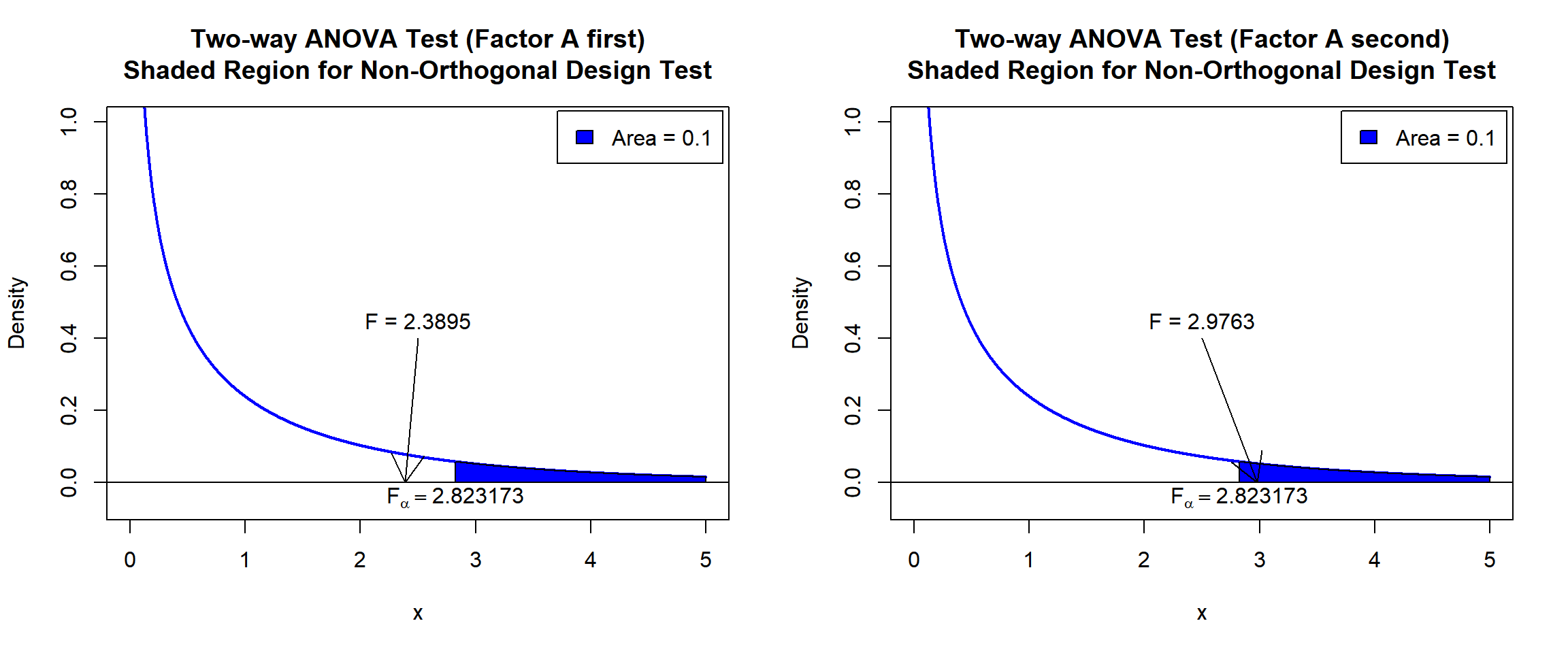

Two-way ANOVA Test Shaded Region for Non-Orthogonal Design Test in R

6 Two-way ANOVA Test: Test Statistics, P-value & Degrees of Freedom in R

Here for a two-way ANOVA test, we show how to get the test statistics (or f-value), sum of squares, mean squares, p-values, and degrees of freedom from the anova() function in R, or by written code.

aov_object1 = anova(lm(uptake ~ Type + Treatment, data = CO2))
aov_object1

Analysis of Variance Table

Response: uptake
          Df Sum Sq Mean Sq F value    Pr(>F)    
Type       1 3365.5  3365.5  50.923 3.679e-10 ***
Treatment  1  988.1   988.1  14.951 0.0002218 ***
Residuals 81 5353.3    66.1                      
---
Signif. codes:  0 '***' 0.001 '**' 0.01 '*' 0.05 '.' 0.1 ' ' 1

Two factors without interaction: test statistic (or f-value), sum of squares, and mean squares:

F-value

For Factor A:

\[\frac {\left[ \sum_{i=1}^r n_{i\cdot}(\bar y_{i\cdot}-\bar y_{\cdot \cdot})^2 \right]/(r-1)}{\left[ \sum_{i=1}^r \sum_{j=1}^c \sum_{k=1}^{n_{ij}} (y_{ijk}-\bar y_{i\cdot}-\bar y_{\cdot j}+\bar y_{\cdot \cdot})^2\right]/(n−r−c+1)}\] For Factor B:

\[\frac {\left[ \sum_{j=1}^c n_{\cdot j}(\bar y_{\cdot j}-\bar y_{\cdot \cdot})^2\right]/(c-1)}{\left[ \sum_{i=1}^r \sum_{j=1}^c \sum_{k=1}^{n_{ij}} (y_{ijk}-\bar y_{i\cdot}-\bar y_{\cdot j}+\bar y_{\cdot \cdot})^2\right]/(n−r−c+1)}\]

aov_object1$`F value`[1:2]

[1] 50.92315 14.95094

Same as (only for orthogonal designs):

y = CO2$uptake; fctA = as.factor(CO2$Type);
fctB = as.factor(CO2$Treatment); intr = fctA:fctB
meansA = tapply(y, fctA, mean) #means
meansB = tapply(y, fctB, mean)
meansintr = tapply(y, intr, mean)
y = y[order(intr)] #order observations by interactions
lensA = tapply(y, fctA, length) #sizes
lensB = tapply(y, fctB, length)
n = length(y); r = length(meansA); c = length(meansB)
ssgA = sum(lensA*(meansA-mean(y))^2) #sum of squares
ssgB = sum(lensB*(meansB-mean(y))^2)
ssr = sum((y - rep(meansA, each = n/r) - rep(meansB, each = n/(r*c), times = r) + mean(y))^2)
numA = ssgA/(r-1); numB = ssgB/(c-1) #mean squares
lenssr = n-(r-1)-(c-1)-1; denom = ssr/lenssr
FA = numA/denom; FB = numB/denom #f-values
c(FA, FB)

[1] 50.92315 14.95094

Sum of squares and mean squares

aov_object1$`Sum Sq`

[1] 3365.5344  988.1144 5353.3268

aov_object1$`Mean Sq`

[1] 3365.53440  988.11440   66.09045

Same as:

#Based on steps above
c(ssgA, ssgB, ssr)

[1] 3365.5344  988.1144 5353.3268

c(numA, numB, denom)

[1] 3365.53440  988.11440   66.09045

To get the p-value:

The p-values are $P (F_{df1, df2}>F_{Observed})$.

aov_object1$`Pr(>F)`[1:2]

[1] 3.679047e-10 2.217501e-04

Same as:

Note that the p-values depend on the $\text{test statistics}$ ($F_{df1, df2} = 50.923$) for factor A, and ($F_{df1, df2} = 14.951$) for factor B; and $\text{degrees of freedom}$ (1, 81) for factor A, and (1, 81) for factor B. We also use the distribution functions pf() for the F distribution in R.

1-pf(50.923, 1, 81)

[1] 3.679225e-10

1-pf(14.951, 1, 81)

[1] 0.0002217442

To get the degrees of freedom:

The degrees of freedom are $\text{df1}=1$ and $\text{df2}=81$ for both factor A and factor B.

aov_object1$Df

[1]  1  1 81

Same as:

r = length(unique(fctA)); c = length(unique(fctB)); n = length(y)
c(r-1, c-1, n-r-c+1)

[1]  1  1 81

7 Two-way ANOVA Test with Interaction Effect: Test Statistics in R

Here for a two-way ANOVA test with interaction effect, we show how to get the test statistics (or f-value), sum of squares, mean squares from the anova() function in R, or by written code.

aov_object2 = anova(lm(uptake ~ Type + Treatment + Type:Treatment, data = CO2))
aov_object2

Analysis of Variance Table

Response: uptake
               Df Sum Sq Mean Sq F value    Pr(>F)    
Type            1 3365.5  3365.5 52.5086 2.378e-10 ***
Treatment       1  988.1   988.1 15.4164 0.0001817 ***
Type:Treatment  1  225.7   225.7  3.5218 0.0642128 .  
Residuals      80 5127.6    64.1                      
---
Signif. codes:  0 '***' 0.001 '**' 0.01 '*' 0.05 '.' 0.1 ' ' 1

Two factors with interaction: test statistic (or f-value), sum of squares, and mean squares:

F-value

For Factor A:

\[\frac {\left[ \sum_{i=1}^r n_{i\cdot}(\bar y_{i\cdot}-\bar y_{\cdot \cdot})^2 \right] /(r-1)}{\left[ \sum_{i=1}^r \sum_{j=1}^c \sum_{k=1}^{n_{ij}} (y_{ijk}-\bar y_{ij})^2 \right] /(n−rc)}\]

For Factor B:

\[\frac {\left[ \sum_{j=1}^c n_{\cdot j}(\bar y_{\cdot j}-\bar y_{\cdot \cdot})^2 \right] /(c-1)}{\left[\sum_{i=1}^r \sum_{j=1}^c \sum_{k=1}^{n_{ij}} (y_{ijk}-\bar y_{ij})^2 \right]/(n−rc)}\]

For AB Interaction:

\[\frac {\left[ \sum_{i=1}^r \sum_{j=1}^c n_{ij}(\bar y_{ij}-\bar y_{i\cdot}-\bar y_{\cdot j}+\bar y_{\cdot \cdot})^2 \right]/(r-1)(c-1)}{\left[ \sum_{i=1}^r \sum_{j=1}^c \sum_{k=1}^{n_{ij}} (y_{ijk}-\bar y_{ij})^2 \right]/(n−rc)}\]

aov_object2$`F value`[1:3]

[1] 52.50856 15.41641  3.52180

Same as (only for orthogonal designs):

y = CO2$uptake; fctA = as.factor(CO2$Type);
fctB = as.factor(CO2$Treatment); intr = fctA:fctB
meansA = tapply(y, fctA, mean) #means
meansB = tapply(y, fctB, mean)
meansintr = tapply(y, intr, mean)
y = y[order(intr)] #order observations by interactions
lensA = tapply(y, fctA, length) #sizes
lensB = tapply(y, fctB, length)
lensintr = tapply(y, intr, length)
n = length(y); r = length(meansA);
c = length(meansB); inl = (r-1)*(c-1)
ssgA = sum(lensA*(meansA-mean(y))^2) #sum of squares
ssgB = sum(lensB*(meansB-mean(y))^2)
ssgintr = sum(lensintr*(meansintr - rep(meansA, each = c) - rep(meansB, times = r) + mean(y))^2)
ssr = sum((y-rep(meansintr, lensintr))^2)
numA = ssgA/(r-1); numB = ssgB/(c-1) #mean squares
numintr = ssgintr/inl
lenssr = n-(r-1)-(c-1)-inl-1; denom = ssr/lenssr
FA = numA/denom; FB = numB/denom; Fintr = numintr/denom #f-values
c(FA, FB, Fintr)

[1] 52.50856 15.41641  3.52180

Sum of squares and mean squares

aov_object2$`Sum Sq`

[1] 3365.5344  988.1144  225.7296 5127.5971

aov_object2$`Mean Sq`

[1] 3365.53440  988.11440  225.72964   64.09496

Same as:

#Based on steps above
c(ssgA, ssgB, ssgintr, ssr)

[1] 3365.5344  988.1144  225.7296 5127.5971

c(numA, numB, numintr, denom)

[1] 3365.53440  988.11440  225.72964   64.09496

Source of Variation	Degrees of Freedom (DF)	Sums of Squares (SS)	Sums of Squares (SS) –ORTHOGONAL DESIGN ONLY–	Mean Square (MS)	F	P-value
Factor A	\(r-1\)	\(SSA\)	\(\sum_{i=1}^r n_{i\cdot}(\bar y_{i\cdot}-\bar y_{\cdot \cdot})^2\)	\(\frac{SSA}{DFA}\)	\(\frac{MSA}{MSR}\)	\(P(F_{r-1 \;,\; n-r-c+1}>F)\)
Factor B	\(c-1\)	\(SSB\)	\(\sum_{j=1}^c n_{\cdot j}(\bar y_{\cdot j}-\bar y_{\cdot \cdot})^2\)	\(\frac{SSB}{DFB}\)	\(\frac{MSB}{MSR}\)	\(P(F_{c-1 \;,\; n-r-c+1}>F)\)
Residuals	\(n-r-c+1\)	\(SSR\)	\(\sum_{i=1}^r \sum_{j=1}^c \sum_{k=1}^{n_{ij}} (y_{ijk}-\bar y_{i\cdot}-\bar y_{\cdot j}+\bar y_{\cdot \cdot})^2\)	\(\frac{SSR}{DFR}\)
Total	\(n-1\)	\(SST\)	\(\sum_{i=1}^r \sum_{j=1}^c \sum_{k=1}^{n_{ij}} (y_{ijk}-\bar y_{\cdot \cdot})^2\)

Source of Variation	Degrees of Freedom (DF)	Sums of Squares (SS)	Sums of Squares (SS) –ORTHOGONAL DESIGN ONLY–	Mean Square (MS)	F	P-value
Factor A	\(r-1\)	\(SSA\)	\(\sum_{i=1}^r n_{i\cdot}(\bar y_{i\cdot}-\bar y_{\cdot \cdot})^2\)	\(\frac{SSA}{DFA}\)	\(\frac{MSA}{MSR}\)	\(P(F_{r-1 \;,\; n−rc}>F)\)
Factor B	\(c-1\)	\(SSB\)	\(\sum_{j=1}^c n_{\cdot j}(\bar y_{\cdot j}-\bar y_{\cdot \cdot})^2\)	\(\frac{SSB}{DFB}\)	\(\frac{MSB}{MSR}\)	\(P(F_{c-1 \;,\; n−rc}>F)\)
Interaction AB	\((r-1)(c-1)\)	\(SSAB\)	\(\sum_{i=1}^r \sum_{j=1}^c n_{ij}(\bar y_{ij}-\bar y_{i\cdot}-\bar y_{\cdot j}+\bar y_{\cdot \cdot})^2\)	\(\frac{SSAB}{DFAB}\)	\(\frac{MSAB}{MSR}\)	\(P(F_{(r-1)(c-1) \;,\; n−rc}>F)\)
Residuals	\(n-rc\)	\(SSR\)	\(\sum_{i=1}^r \sum_{j=1}^c \sum_{k=1}^{n_{ij}} (y_{ijk}-\bar y_{ij})^2\)	\(\frac{SSR}{DFR}\)
Total	\(n-1\)	\(SST\)	\(\sum_{i=1}^r \sum_{j=1}^c \sum_{k=1}^{n_{ij}} (y_{ijk}-\bar y_{\cdot \cdot})^2\)

	Factor B (Column Factor)
Factor A (Row Factor)		Column 1	Column 2	\(\cdots\)	Column \(c\)	Aggregate
	Row 1	\(\bar y_{11}\) \(n_{11}\)	\(\bar y_{12}\) \(n_{12}\)	\(\cdots\)	\(\bar y_{1c}\) \(n_{1c}\)	\(\bar y_{1\cdot}\) = Row Mean \(n_{1\cdot}\) = Row Size
	Row 2	\(\bar y_{21}\) \(n_{21}\)	\(\bar y_{22}\) \(n_{22}\)	\(\cdots\)	\(\bar y_{2c}\) \(n_{2c}\)	\(\bar y_{2\cdot}\) = Row Mean \(n_{2\cdot}\) = Row Size
	\(\vdots\)	\(\vdots\)	\(\vdots\)	\(\ddots\)	\(\vdots\)	\(\vdots\)
	Row \(r\)	\(\bar y_{r1}\) \(n_{r1}\)	\(\bar y_{r2}\) \(n_{r2}\)	\(\cdots\)	\(\bar y_{rc}\) \(n_{rc}\)	\(\bar y_{r\cdot}\) = Row Mean \(n_{r\cdot}\) = Row Size
	Aggregate	\(\bar y_{\cdot1}\) = Col Mean \(n_{\cdot1}\) = Col Size	\(\bar y_{\cdot2}\) = Col Mean \(n_{\cdot2}\) = Col Size	\(\cdots\)	\(\bar y_{\cdot c}\) = Col Mean \(n_{\cdot c}\) = Col Size	\(\bar y_{\cdot \cdot}\) = Grand Mean \(n\) = Total Size

Factor A	Factor B
\(H_0:\) there is no effect from Factor A \((\mu_{1\cdot} = \mu_{2\cdot} = \mu_{3\cdot})\).	\(H_0:\) there is no effect from Factor B \((\mu_{\cdot 1} = \mu_{\cdot 2})\).
\(H_1:\) at least one group’s mean is different, hence, an effect.	\(H_1:\) at least one group’s mean is different, hence, an effect.

Factor A	Factor B
The test statistic, \(F\), is 4.8366,	The test statistic, \(F\), is 1.6476,
the degrees of freedom, are numerator df \(r-1= 2\), denominator df \(n-r-c+1= 20\),	the degrees of freedom, are numerator df \(c-1= 1\), denominator df \(n-r-c+1= 20\),
the p-value, \(p\), is 0.01935.	the p-value, \(p\), is 0.21396.

Factor A	Factor B
P-value: With the p-value \((p = 0.01935)\) being less than the level of significance 0.05, we reject the null hypothesis that there is no effect from Factor A.	P-value: With the p-value \((p = 0.21396)\) being greater than the level of significance 0.05, we fail to reject the null hypothesis that there is no effect from Factor B.
\(F\) T-statistic: With test statistics value \((F_{2, 20} = 4.8366)\) being in the critical region (shaded area), that is, \(F_{2, 20} = 4.8366\) greater than \(F_{2, 20, \alpha}=\text{qf(0.95, 2, 20)}\)\(=3.4928285\), we reject the null hypothesis that there is no effect from Factor A.	\(F\) T-statistic: With test statistics value \((F_{1, 20} = 1.6476)\) being less than the critical value, \(F_{1, 20, \alpha}=\text{qf(0.95, 1, 20)}\)\(=4.3512435\) (or not in the shaded region), we fail to reject the null hypothesis that there is no effect from Factor B.

Factor A	Factor B	Interaction AB
\(H_0:\) there is no effect from Factor A \((\mu_{1\cdot} = \mu_{2\cdot})\).	\(H_0:\) there is no effect from Factor B \((\mu_{\cdot 1} = \mu_{\cdot 2} = \mu_{\cdot 3})\).	\(H_0:\) there is no interaction effect \((\mu_{ij}-\mu_{i\cdot}-\mu_{\cdot j}\), for each cell \(ij\) are all equal).
\(H_1:\) at least one group’s mean is different, hence, an effect.	\(H_1:\) at least one group’s mean is different, hence, an effect.	\(H_1:\) at least one interaction’s net mean is different, hence, an effect.

Test 1	Test 2
P-value: With the p-value \((p = 0.129314)\) being greater than the level of significance 0.1, we fail to reject the null hypothesis that there is no effect from Factor A.	P-value: With the p-value \((p = 0.091511)\) being less than the level of significance 0.1, we reject the null hypothesis that there is no effect from Factor A after accounting for Factor B effects.
\(F\) T-statistic: With test statistics value \((F_{1, 44} = 2.3895)\) being less than the critical value, \(F_{1, 44, \alpha}=\text{qf(0.9, 1, 44)}\)\(=2.8231728\) (or not in the shaded region), we fail to reject the null hypothesis that there is no effect from Factor A accounting for Factor A effects first.	\(F\) T-statistic: With test statistics value \((F_{1, 44} = 2.9763)\) being in the critical region (shaded area), that is, \(F_{1, 44} = 2.9763\) greater than \(F_{1, 44, \alpha}=\text{qf(0.9, 1, 44)}\)\(=2.8231728\), we reject the null hypothesis that there is no effect from Factor A accounting for Factor B effects first.

Two-way ANOVA Tests in R

Sample Steps to Run a Two-way ANOVA Test:

Creating a Two-way ANOVA Test Object:

1 Test Statistic for Two-way ANOVA Test in R

Notations

Notations Table

2 Simple Two-way ANOVA Test in R

Interpretation:

3 Two-way ANOVA Test Critical Value in R

4 Two-way ANOVA Test with Interaction Effect in R

Interpretation:

5 Two-way ANOVA Test for Non-Orthogonal Design in R

6 Two-way ANOVA Test: Test Statistics, P-value & Degrees of Freedom in R

Two factors without interaction: test statistic (or f-value), sum of squares, and mean squares:

F-value

Sum of squares and mean squares

To get the p-value:

To get the degrees of freedom:

7 Two-way ANOVA Test with Interaction Effect: Test Statistics in R

Two factors with interaction: test statistic (or f-value), sum of squares, and mean squares:

F-value

Sum of squares and mean squares