Zero Intercept Regression in R
Here, we discuss how to force a zero intercept in regression in R with interpretations, including coefficients, r-squared, and p-values.
Linear regression with zero intercept can be performed in R with the
lm() function from the "stats" package in the base
version of R.
The zero intercept regression with the assumption that the regression line passes through the origin can be used to study the linear relationship, if one exists, between a dependent variable \((y)\) and an independent variable \((x)\). Hence, when the independent variable is 0, the dependent variable is also 0.
For cases of multiple independent variables, the zero intercept regression assumes that the dependent variable \((y)\) is 0 when all the independent variables \((x's)\) are also equal to 0.
The zero intercept regression framework is based on the theoretical assumption that, \[y = \beta x + \varepsilon,\]
or, for multiple independent variables,
\[y = \beta_1 x_1 + \beta_2 x_2 + \cdots + \beta_p x_p + \varepsilon,\]
where \(\varepsilon\) represents the error terms that are 1) independent, 2) normal distributed, 3) have constant variance, and 4) have mean zero.
The zero intercept regression model estimates the true coefficients, \(\beta_k\), as \(\widehat \beta_k\). Then for any \(x\) value, these are used to predict or estimate the true \(y\), as \(\widehat y\), with the equations below:
\[\widehat y = \widehat \beta x,\]
or, for multiple independent variables,
\[\widehat y = \widehat \beta_1 x_1 + \widehat \beta_2 x_2 + \cdots + \widehat \beta_p x_p.\]
For non-zero intercept, see simple linear regression and multiple linear regression.
Sample Steps to Run a Zero Intercept Regression:
# Create the data samples for the regression model
# Values are paired based on matching position in each sample

x = c(3.5, 2.9, 3.2, 2.1, 1.7, 4.4, 3.3, 2.6)
y = c(6.3, 5.2, 6.3, 5.1, 3.5, 8.4, 6.7, 5.5)
df_data = data.frame(y, x)
df_data

# Run the regression model forcing the intercept to zero with "-1"

model = lm(y ~ -1 + x)
summary(model)

#or

model = lm(y ~ -1 + x, data = df_data)
summary(model)
y x
1 6.3 3.5
2 5.2 2.9
3 6.3 3.2
4 5.1 2.1
5 3.5 1.7
6 8.4 4.4
7 6.7 3.3
8 5.5 2.6
Call:
lm(formula = y ~ -1 + x)

Residuals:
    Min      1Q  Median      3Q     Max
-0.5557 -0.2841  0.1010  0.2788  0.9866

Coefficients:
  Estimate Std. Error t value Pr(>|t|)
x  1.95878    0.05867   33.39  5.6e-09 ***
---
Signif. codes:  0 '***' 0.001 '**' 0.01 '*' 0.05 '.' 0.1 ' ' 1

Residual standard error: 0.5088 on 7 degrees of freedom
Multiple R-squared:  0.9938,    Adjusted R-squared:  0.9929
F-statistic: 1115 on 1 and 7 DF, p-value: 5.602e-09| Argument | Usage |
| y ~ -1 + x | y is the dependent sample, and x is the independent sample |
| y ~ -1 + x1 +…+ xp | y is the dependent sample, and x1, x2, …, xp are the independent samples |
| data | The dataframe object that contains the dependent and independent variables |
1 Steps to Running a Zero Intercept Regression in R
Using the rock data from the "datasets" package with 10 sample rows from 48 rows below:
    area     peri     shape  perm
1   4990 2791.900 0.0903296   6.3
6   7979 4010.150 0.1670450  17.1
10  6425 3098.650 0.1623940 119.0
17 10962 4608.660 0.2043140  58.6
23 12212 4697.650 0.2400770 142.0
29  6509 1851.210 0.2252140 890.0
38  1468  476.322 0.4387120 100.0
39  3524 1189.460 0.1635860 100.0
46  1651  597.808 0.2626510 580.0
48  9718 1485.580 0.2004470 580.0
NOTE: The dependent variable is "area", and the independent variable is "peri".
1.1 Check for Linear Relationship Through the Origin
We can visually check for a zero intercept linear relationship based on a scatter plot and a line through the origin.
x = rock$peri
y = rock$area
plot(x, y,
     xlim = c(0, max(x)), ylim = c(0, max(y)),
     main = "Scatter Plot with Zero Intercept Regression
and Lowess Lines in R")
abline(lm(y ~ -1 + x), col = "blue")
lines(lowess(x, y), col = "red", lty = "dashed")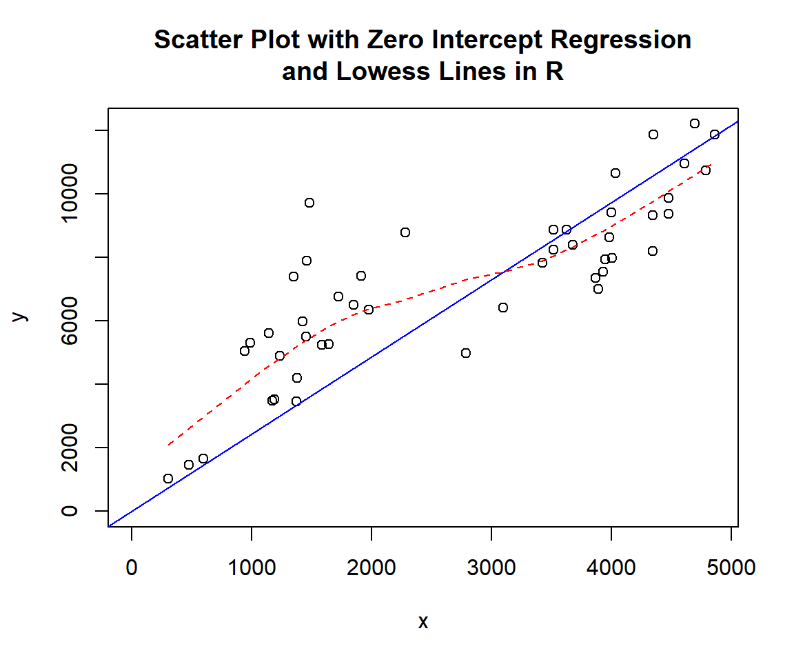
Scatter Plot with Zero Intercept Regression and Lowess Lines in R
The appearance of the scatter plot with zero intercept regression line (blue) suggests a strong linear relationship, and the line is also close to the lowess line (red).
1.2 Run the Zero Intercept Regression
Run the zero intercept regression model with the regression line
through the origin, by using the argument "-1" in the lm()
function, and print the results using the summary()
function.
peri = rock$peri
area = rock$area

# Regression without the intercept term
model = lm(area ~ -1 + peri)
summary(model)
Or:
Call:
lm(formula = area ~ -1 + peri, data = rock)

Residuals:
    Min      1Q  Median      3Q     Max
-2463.2  -930.1   311.7  1982.3  6105.7

Coefficients:
     Estimate Std. Error t value Pr(>|t|)
peri  2.43159    0.09987   24.35   <2e-16 ***
---
Signif. codes:  0 '***' 0.001 '**' 0.01 '*' 0.05 '.' 0.1 ' ' 1

Residual standard error: 2099 on 47 degrees of freedom
Multiple R-squared:  0.9265,    Adjusted R-squared:  0.925
F-statistic: 592.8 on 1 and 47 DF,  p-value: < 2.2e-16
1.3 Interpretation of the Results
Coefficients:
The estimated coefficient for \(x\) (\(\widehat \beta\)) is \(\text{summary(model)\$coefficients[1, 1]}\) \(= 2.432\).P-values:
- The p-value for the independent variable, \(x\) (peri), is \(\text{summary(model)\$coefficients[1, 4]}\) \(\approx 0\).
- For level of significance, \(\alpha = 0.05\), since the p-value is less than \(0.05\), we say that the independent variable is a statistically significant predictor of the dependent variable \(y\) (area).
R-squared:
The r-squared value is \(\text{summary(model)\$r.squared}\) \(= 0.927\).
This means that the model, using the independent variable, \(x\) (peri), explains \(92.7\%\) of the variations in the dependent variable \(y\) (area) from the origin (0).
1.4 Prediction and Estimation
To predict or estimate \(y\) for any \(x\), we can use \(y = 2.432 x\).
For example, for \(x = 2000\), \(y = 2.432 \times 2000\) \(= 4864\).
2 Zero Intercept Regression with Multiple Variables in R
Using the attitude data from the "datasets" package with 10 sample rows from 30 rows below:
   rating complaints privileges learning raises critical advance
1      43         51         30       39     61       92      45
4      61         63         45       47     54       84      35
5      81         78         56       66     71       83      47
7      58         67         42       56     66       68      35
12     67         60         47       39     59       74      41
17     74         85         64       69     79       79      63
19     65         70         46       57     75       85      46
20     50         58         68       54     64       78      52
23     53         66         52       50     63       80      37
30     82         82         39       59     64       78      39
NOTE: The dependent variable is "rating".
Run the Zero Intercept Regression for Multiple Variables
Run the multiple regression without the intercept term by using the
argument "-1" in the lm() function, and print the results
using the summary() function.
# Regression without the intercept term
model = lm(rating ~ -1 + complaints + privileges,
           data = attitude)
summary(model)
Call:
lm(formula = rating ~ -1 + complaints + privileges, data = attitude)

Residuals:
    Min      1Q  Median      3Q     Max
-12.687  -6.613   2.191   6.098  12.477

Coefficients:
           Estimate Std. Error t value Pr(>|t|)
complaints  0.92659    0.10398   8.911 1.15e-09 ***
privileges  0.04554    0.12955   0.352    0.728
---
Signif. codes:  0 '***' 0.001 '**' 0.01 '*' 0.05 '.' 0.1 ' ' 1

Residual standard error: 7.543 on 28 degrees of freedom
Multiple R-squared:  0.9877,    Adjusted R-squared:  0.9868
F-statistic:  1125 on 2 and 28 DF,  p-value: < 2.2e-16
Interpretation of the Regression Results
- Coefficients:
- The estimated coefficient for \(x_1\) (\(\widehat \beta_1\)) is \(\text{summary(model)\$coefficients[1, 1]}\) \(= 0.927\).
- The estimated coefficient for \(x_2\) (\(\widehat \beta_2\)) is \(\text{summary(model)\$coefficients[2, 1]}\) \(= 0.046\).
- P-values:
For level of significance, \(\alpha = 0.05\).- The p-value for the independent variable, \(x_1\) (complaints), is \(\text{summary(model)\$coefficients[1, 4]}\) \(= 1.2\times 10^{-9}\). Since the p-value is less than \(0.05\), we say that \(x_1\) is a statistically significant predictor of the dependent variable \(y\) (rating).
- For \(x_2\) (privileges), it is \(\text{summary(model)\$coefficients[2, 4]}\) \(= 0.728\). Since the p-value is greater than \(0.05\), we say that \(x_2\) is NOT a statistically significant predictor of the dependent variable \(y\) (rating) in the presence of \(x_1\) (complaints).
- R-squared:
The r-squared value is \(\text{summary(model)\$r.squared}\) \(= 0.988\). This means that the model, using the independent variables, \(x_1\) and \(x_2\) (complaints and privileges), explains \(98.8\%\) of the variations in the dependent variable \(y\) (rating) from the origin (0).
Prediction and Estimation
To predict or estimate \(y\) for any \(x_1\) and \(x_2\), we can use \(y = 0.927 x_1 + 0.046 x_2\).
For example, for \(x_1 = 60\) and \(x_2 = 50\), \(y = 0.927 \times 60 + 0.046 \times 50\) \(= 57.92\).
The feedback form is a Google form but it does not collect any personal information.
Please click on the link below to go to the Google form.
Thank You!
Go to Feedback Form
Copyright © 2020 - 2026. All Rights Reserved by Stats Codes