Binomial Distributions in R
- 1 Table of Binomial Distribution Functions in R
- 2 Plot of Binomial Distributions in R
- 3 Examples for Setting Parameters for Binomial Distributions in R
- 4 rbinom(): Random Sampling from Binomial Distributions in R
- 5 dbinom(): Probability Mass Function for Binomial Distributions in R
- 6 pbinom(): Cumulative Distribution Function for Binomial Distributions in R
- 7 qbinom(): Derive Quantile for Binomial Distributions in R
Here, we discuss binomial distribution functions in R, plots, parameter setting, random sampling, mass function, cumulative distribution and quantiles.
The binomial distribution for the number of successes in a sequence of independent and identically distributed \(n\) Bernoulli trials, with parameters \(\tt{size}=n\), and \(\tt{probability\:of\:success}=p\) has probability mass function (pmf) formula as:
\[P(X=x)=\binom{n}{x} p^x q^{n-x} = \frac{n!}{x!(n-x)!} p^x q^{n-x},\] for \(x \in \{0, 1, \ldots, n\}\) number of successes,
where \(n \in \{0, 1, 2, \ldots\}\) is the number of trials,
\(p \in [0,1]\) is the probability of success in each trial,
the \(\tt{binomial\; coefficient}\) \(\binom{a}{b}\) equals \(\frac{a!}{b!(a-b)!}\),
and \(a!\), the \(\tt{factorial\; operator}\), equals \(a\times(a-1)\times(a-2)\times\cdots\times 1\).
The mean is \(np\), and the variance is \(npq\).
See also probability distributions and plots and charts.
1 Table of Binomial Distribution Functions in R
The table below shows the functions for binomial distributions in R.
| Function | Usage |
| rbinom(n, size, prob) | Simulate a random sample with \(n\) observations |
| dbinom(x, size, prob) | Calculate the probability mass at the point \(x\) |
| pbinom(q, size, prob) | Calculate the cumulative distribution at the point \(q\) |
| qbinom(p, size, prob) | Calculate the quantile value associated with \(p\) |
2 Plot of Binomial Distributions in R
Single distribution:
Below is a plot of the binomial distribution function with \(\tt{size}=20\), and \(\tt{probability\:of\:success}=0.6\).
x = 0:20; y = dbinom(x, 20, 0.6)
plot(x, y, type = "h",
     xlim = c(0, 20), ylim = c(0, max(y)),
     main = "Probability Mass Function of
Binomial Distribution (20, 0.6)",
     xlab = "x", ylab = "Mass",
     col = "blue")
# Add legend
legend("topleft", "size = 20, prob = 0.6",
       fill = "blue",
       bty = "n")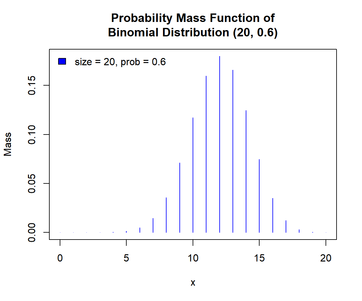
Probability Mass Function (PMF) of a Binomial Distribution in R
Multiple distributions:
Below is a plot of multiple binomial distribution functions in one graph.
x1 = 0:30; y1 = dbinom(x1, 30, 0.6)
x2 = 0:30; y2 = dbinom(x2, 30, 0.3)
x3 = 0:20; y3 = dbinom(x3, 20, 0.6)
plot(x1, y1,
     xlim = c(0, 30), ylim = range(c(y1, y2, y3)),
     main = "Probability Mass Functions of Binomial Distributions",
     xlab = "x", ylab = "Mass",
     col = "blue")
points(x2, y2, col = "red")
points(x3, y3, col = "green")
# Add legend
legend("topright", c("size = 30, prob = 0.6",
                    "size = 30, prob = 0.3",
                    "size = 20, prob = 0.6"),
       fill = c("blue", "red", "green"),
       bty = "n")
# Add lines
for(i in 1:30){
  segments(x1[i], dbinom(x1[i], 30, 0.6),
           x1[i+1], dbinom(x1[i+1], 30, 0.6),
           col = "blue")}
for(i in 1:30){
  segments(x2[i], dbinom(x2[i], 30, 0.3),
           x2[i+1], dbinom(x2[i+1], 30, 0.3),
           col = "red")}
for(i in 1:20){
  segments(x3[i], dbinom(x3[i], 20, 0.6),
           x3[i+1], dbinom(x3[i+1], 20, 0.6),
           col = "green")}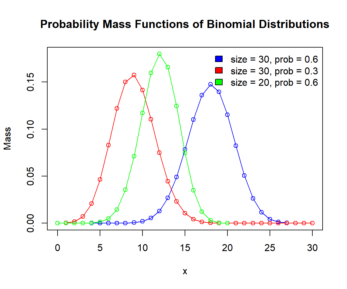
Probability Mass Functions (PMFs) of Binomial Distributions in R
3 Examples for Setting Parameters for Binomial Distributions in R
To set the parameters for the binomial distribution function, with \(\tt{size}=10\) and \(\tt{probability\:of\:success}=0.5\).
For example, for dbinom(), the following are the
same:
# The order of 10 and 0.5 matters here as the parameter names are not used.
# The first number 10 is size, and 0.5 is prob.
dbinom(2, 10, 0.5)
[1] 0.04394531[1] 0.04394531[1] 0.043945314 rbinom(): Random Sampling from Binomial Distributions in R
Sample 800 observations from the binomial distribution with \(\tt{size}=25\) and \(\tt{probability\:of\:success}=0.4\):
set.seed(12) # Line allows replication (use any number).
sample = rbinom(800, 25, 0.4)
hist(sample,
     main = "Histogram of 800 Observations from
Binomial Distribution with Size = 25 and Prob = 0.4",
     xlab = "x",
     col = "lightblue", border = "white")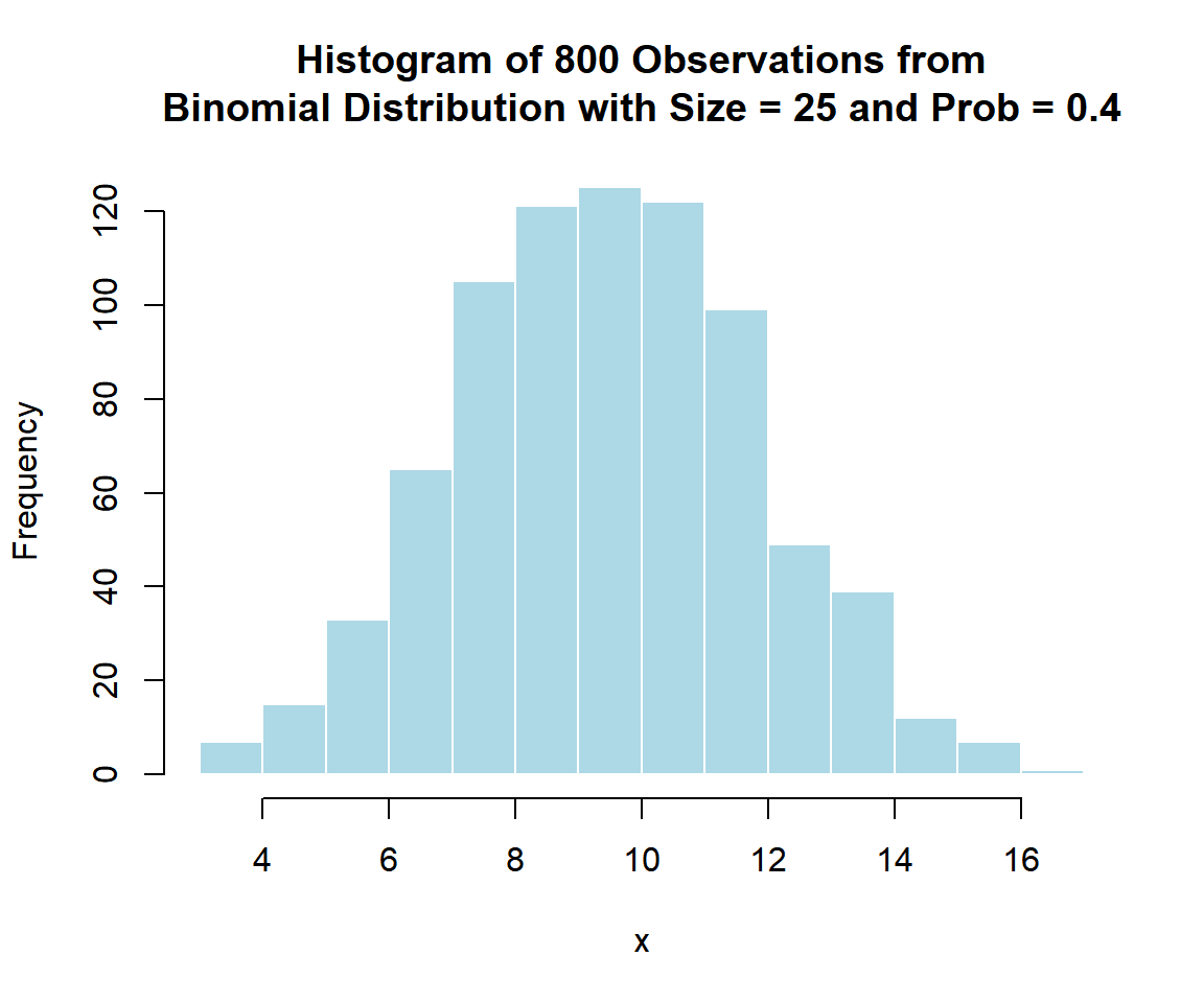
Histogram of Binomial Distribution (25, 0.4) Random Sample in R
5 dbinom(): Probability Mass Function for Binomial Distributions in R
Calculate the mass at \(x = 14\), in the binomial distribution with \(\tt{size}=18\) and \(\tt{probability\:of\:success}=0.65\):
[1] 0.1103521x = 0:18; y = dbinom(x, 18, 0.65)
plot(x, y,
xlim = c(0, 18), ylim = c(0, max(y)),
main = "Probability Mass Function of Binomial Distribution
with Size = 18 and Prob = 0.65",
xlab = "x", ylab = "Mass",
col = "blue")
# Add lines
segments(14, -1, 14, 0.1103521)
segments(-1, 0.1103521, 14, 0.1103521)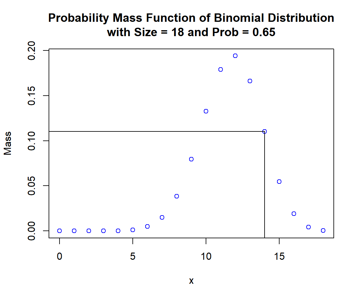
Probability Mass Function (PMF) of Binomial Distribution (18, 0.65) in R
6 pbinom(): Cumulative Distribution Function for Binomial Distributions in R
Calculate the cumulative distribution at \(x = 7\), in the binomial distribution with \(\tt{size}=14\) and \(\tt{probability\:of\:success}=0.4\). That is, \(P(X \le 7)\):
[1] 0.8498599x = 0:14; y = pbinom(x, 14, 0.4)
plot(x, y,
xlim = c(0, 14), ylim = c(0, 1),
main = "Cumulative Distribution Function of Binomial Distribution
with Size = 14 and Prob = 0.4",
xlab = "x", ylab = "Cumulative Distribution",
col = "blue")
# Add lines
for(i in 1:14){
segments(x[i], pbinom(x[i], 14, 0.4),
x[i] + 1, pbinom(x[i], 14, 0.4),
col = "blue")
}
segments(7, -1, 7, 0.8498599)
segments(-1, 0.8498599, 7, 0.8498599)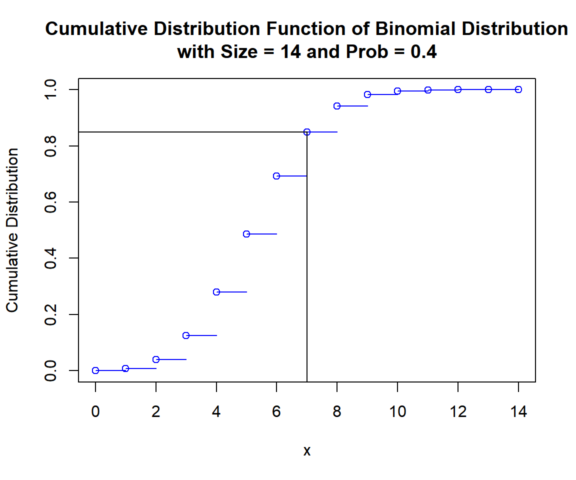
Cumulative Distribution Function (CDF) of Binomial Distribution (14, 0.4) in R
For upper tail, at \(x = 7\), that is, \(P(X > 7) = 1 - P(X \le 7)\), set the "lower.tail" argument:
[1] 0.15014017 qbinom(): Derive Quantile for Binomial Distributions in R
Derive the quantile for \(p = 0.9\), in the binomial distribution with \(\tt{size}=12\) and \(\tt{probability\:of\:success}=0.5\). That is, the \(\tt{smallest}\) \(x\) such that, \(P(X\le x) \ge 0.9\):
[1] 8x = 0:12; y = pbinom(x, 12, 0.5)
plot(x, y,
xlim = c(0, 12), ylim = c(0, 1),
main = "Cumulative Distribution Function of Binomial Distribution
with Size = 12 and Prob = 0.5",
xlab = "x", ylab = "Cumulative Distribution",
col = "blue")
# Add lines
for(i in 1:12){
segments(x[i], pbinom(x[i], 12, 0.5),
x[i] + 1, pbinom(x[i], 12, 0.5),
col = "blue")
}
segments(8, -1, 8, 0.9)
segments(-1, 0.9, 8, 0.9)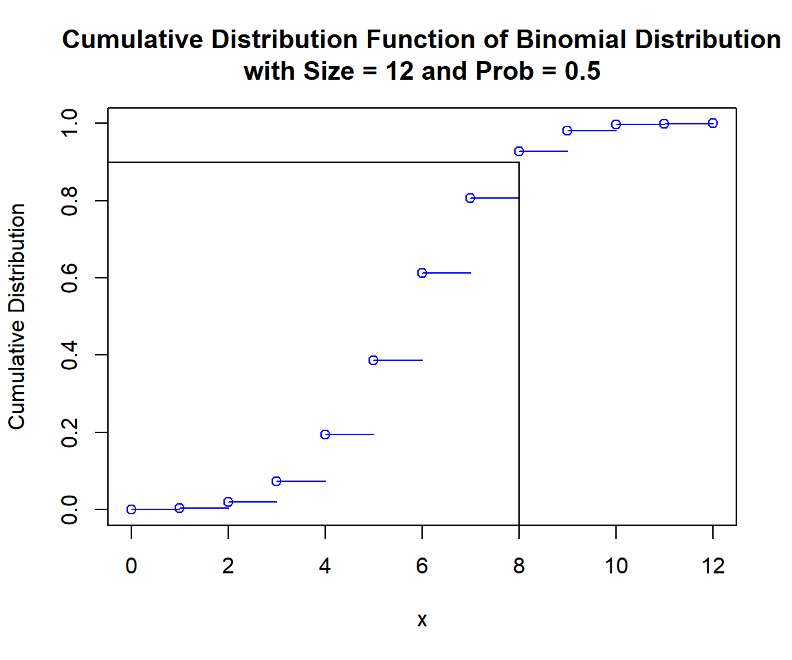
Cumulative Distribution Function (CDF) of Binomial Distribution (12, 0.5) in R
For upper tail, for \(p = 0.10\), that is, the \(\tt{smallest}\) \(x\) such that, \(P(X > x) < 0.1\):
Note: \(P(X > x) = 1-P(X \le x)\).
[1] 8The feedback form is a Google form but it does not collect any personal information.
Please click on the link below to go to the Google form.
Thank You!
Go to Feedback Form
Copyright © 2020 - 2026. All Rights Reserved by Stats Codes