1 Test Statistic for One Variance Chi-squared Test in R
2 Simple One Variance Chi-squared Test in R
3 One Variance Chi-squared Test Critical Value in R
4 Two-tailed One Variance Chi-squared Test in R
5 One-tailed One Variance Chi-squared Test in R
6 One Variance Chi-squared Test: Test Statistics, P-value & Degree of Freedom in R
7 One Variance Chi-squared Test: Estimate & Confidence Interval in R

Here, we discuss the one variance chi-squared test in R with interpretations, including, chi-squared value, p-values, critical values, and confidence intervals.

The one variance chi-squared test in R can be performed with the VarTest() function from the "DescTools" package.

The one variance chi-squared test can be used to test whether the variance of the population were an independent random sample comes from is equal to a certain value (stated in the null hypothesis) or not.

In the one variance chi-squared test, the test statistic follows a chi-squared distribution when the null hypothesis is true.

One Variance Chi-squared Tests & Hypotheses
Question	Is the variance equal to $\sigma_0$?	Is the variance greater than $\sigma_0$?	Is the variance less than $\sigma_0$?
Form of Test	Two-tailed	Right-tailed test	Left-tailed test
Null Hypothesis, $H_0$	$\sigma = \sigma_0$	$\sigma = \sigma_0$	$\sigma = \sigma_0$
Alternate Hypothesis, $H_1$	$\sigma \neq \sigma_0$	$\sigma > \sigma_0$	$\sigma < \sigma_0$

Install and Load the "DescTools" Package:

To use the VarTest() function form the "DescTools" package, first install the package, then load it as follows:

install.packages("DescTools")

library(DescTools)

Sample Steps to Run a One Variance Chi-squared Test:

# After installing and loading the DescTools package as above.

# Create the data for the one variance chi-squared test

data = c(10.9, 8.2, 5.7, 8.7, 6.2)

# Run the one variance chi-squared test with specifications

VarTest(data, sigma.squared = 4,
        alternative = "two.sided",
        conf.level = 0.95)


    One Sample Chi-Square test on variance

data:  data
X-squared = 4.363, df = 4, p-value = 0.4076
alternative hypothesis: true variance is not equal to 4
95 percent confidence interval:
  1.566145 36.026696
sample estimates:
variance of x 
        4.363

Table of Some One Variance Chi-squared Tests Arguments in R
Argument	Usage
x	The sample data values
sigma.squared	The value of the population variance in the null hypothesis
alternative	Set alternate hypothesis as "greater", "less", or the default "two.sided"
conf.level	Level of confidence for the test and confidence interval (default = 0.95)

Creating a One Variance Chi-squared Test Object:

# After installing and loading the DescTools package as above.

# Create data
data = rnorm(100, 0, 2)

# Create object
var_object = VarTest(data, sigma.squared = 4,
                     alternative = "two.sided",
                     conf.level = 0.95)

# Extract a component
var_object$statistic

X-squared 
 82.49005

Table of Some One Variance Chi-squared Test Object Outputs in R
Test Component	Usage
var_object$statistic	Test-statistic value
var_object$p.value	P-value
var_object$parameter	Degrees of freedom
var_object$estimate	Point estimate or sample variance
var_object$conf.int	Confidence interval

1 Test Statistic for One Variance Chi-squared Test in R

The one variance chi-squared test has test statistics, $\chi^2$, of the form:

\[\chi^2 = \frac{(n-1)s^2}{\sigma_0^2}.\]

For an independent random sample that comes from a normal distribution, $\chi^2$ is said to follow the chi-squared distribution ($\chi^2_{n-1}$) when the null hypothesis is true, with $n - 1$ degrees of freedom.

$s^2$ is the sample variance,

$\sigma^2_0$ is the population variance to be tested and set in the null hypothesis,

and $n$ is the sample size.

2 Simple One Variance Chi-squared Test in R

Enter the data by hand.

data = c(19.53, 19.95, 19.18, 20.12, 20.91,
         23.16, 20.47, 20.38, 19.38, 19.77,
         20.86, 19.70, 19.23, 19.68, 21.10)

The sample variance is $s^2 = 1.0344029$ (var(data)).

For the following null hypothesis $H_0$, and alternative hypothesis $H_1$, with the level of significance $\alpha=0.05$.

$H_0:$ the population variance is equal to 1 ($\sigma^2 = 1$).

$H_1:$ the population variance is not equal to 1 ($\sigma^2 \neq 1$, hence the default two-sided).

Because the level of significance is $\alpha=0.05$, the level of confidence is $1 - \alpha = 0.95$.

The VarTest() function has the default variance as 1, the default alternative as "two.sided", and the default level of confidence as 0.95, hence, you do not need to specify the "sigma.squared", "alternative", and "conf.level" arguments in this case.

VarTest(data, sigma.squared = 1,
        alternative = "two.sided",
        conf.level = 0.95)

Or:

VarTest(data)


    One Sample Chi-Square test on variance

data:  data
X-squared = 14.482, df = 14, p-value = 0.6392
alternative hypothesis: true variance is not equal to 1
95 percent confidence interval:
 0.5544496 2.5728095
sample estimates:
variance of x 
     1.034403

The test statistic, $\chi^2$, is 14.482,

the degrees of freedom $n-1$, is 14

the p-value, $p$, is 0.6392,

the 95% confidence interval is [0.5544496, 2.5728095].

Interpretation:

Note that for two-tailed tests from the VarTest() in R, the one variance chi-squared test’s p-value method may disagree with the T-statistic and confidence interval methods for some edge cases. This is because the p-value is based on theoretical considerations due to asymmetry of the chi-squared distribution, while the T-statistic and confidence interval are based on areas of size $\alpha/2$ in the right and left tails.

P-value: With the p-value ($p = 0.6392$) being greater than the level of significance 0.05, we fail to reject the null hypothesis that the population variance is equal to 1.
$\chi^2$ T-statistic: With test statistics value ($\chi^2_{14} = 14.482$) being between the critical values, $\chi^2_{14, \alpha/2}=\text{qchisq(0.025, 14)}$$=5.6287261$ and $\chi^2_{14, 1-\alpha/2}=\text{qchisq(0.975, 14)}$$=26.118948$ (or not in the shaded region), we fail to reject the null hypothesis that the population variance is equal to 1.
Confidence Interval: With the null hypothesis population variance ($\sigma^2 = 1$) being inside the confidence interval, $[0.5544496, 2.5728095]$, we fail to reject the null hypothesis that the population variance is equal to 1.

x = seq(0.01, 35, 1/1000); y = dchisq(x, df=14)
plot(x, y, type = "l",
     xlim = c(0, 35), ylim = c(-0.006, min(max(y), 1)),
     main = "One Variance Chi-squared Test
Shaded Region for Simple Test",
     xlab = "x", ylab = "Density",
     lwd = 2, col = "blue")
abline(h=0)
# Add shaded region and legend
point1 = qchisq(0.025, 14); point2 = qchisq(0.975, 14)
polygon(x = c(0, x[x <= point1], point1),
        y = c(0, y[x <= point1], 0),
        col = "blue")
polygon(x = c(x[x >= point2], 35, point2),
        y = c(y[x >= point2], 0, 0),
        col = "blue")
legend("topright", c("Area = 0.05"),
       fill = c("blue"), inset = 0.01)
# Add critical value and Chi-squared value
arrows(14.482, 0.01, 14.482, 0)
text(14.482, 0.015, "Chi-squared = 14.482")
text(5.628726, -0.004, expression(chi[n-1][','][alpha/2]^2==5.628726))
text(26.11895, -0.004, expression(chi[n-1][','][1-alpha/2]^2==26.11895))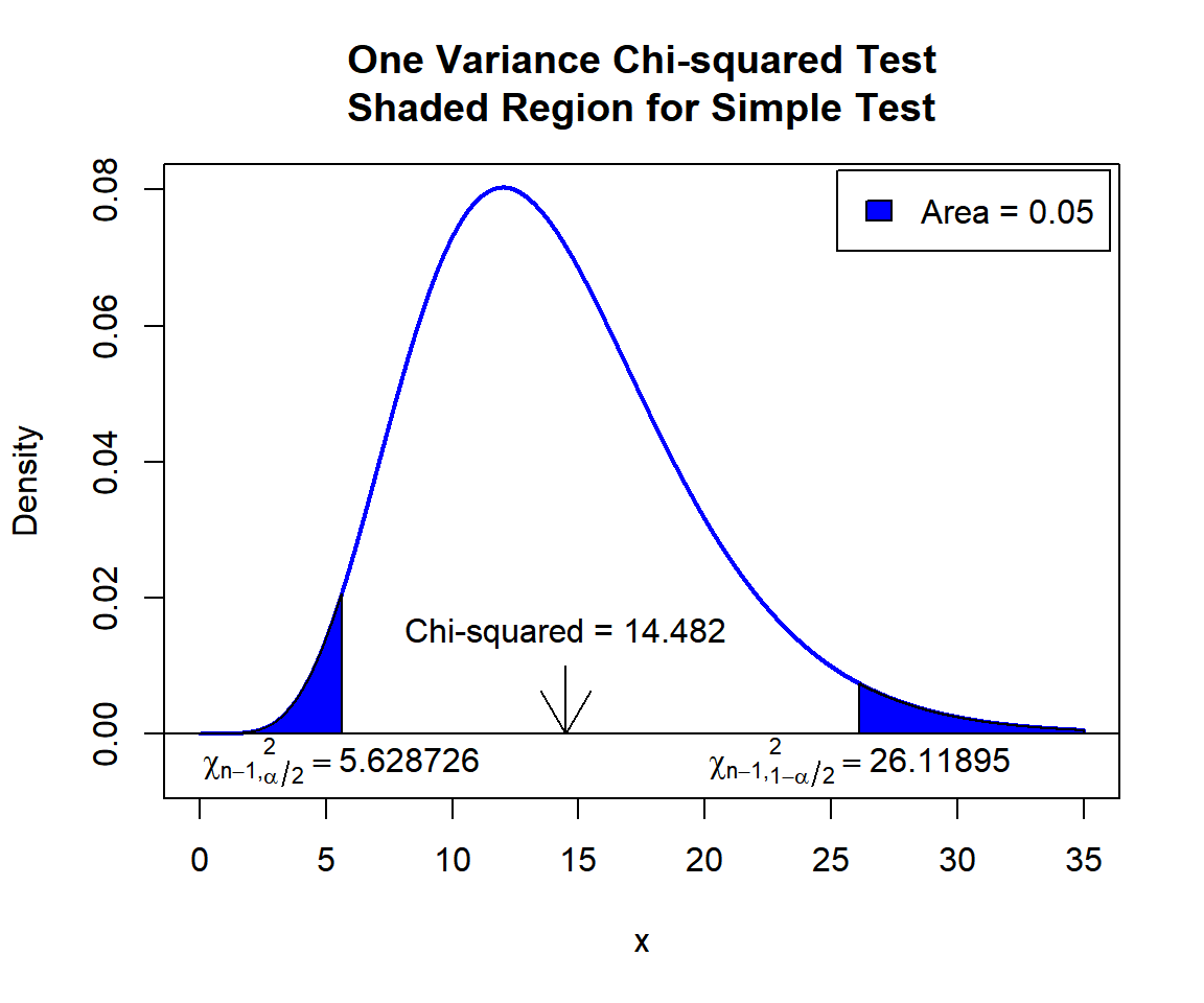

One Variance Chi-squared Test Shaded Region for Simple Test in R

See line charts, shading areas under a curve, lines & arrows on plots, mathematical expressions on plots, and legends on plots for more details on making the plot above.

3 One Variance Chi-squared Test Critical Value in R

To get the critical value for a one variance chi-squared test in R, you can use the qchisq() function for chi-squared distribution to derive the quantile associated with the given level of significance value $\alpha$.

For two-tailed test with level of significance $\alpha$. The critical values are: qchisq($\alpha/2$, df) and qchisq($1-\alpha/2$, df).

For one-tailed test with level of significance $\alpha$. The critical value is: for left-tailed, qchisq($\alpha$, df); and for right-tailed, qchisq($1-\alpha$, df).

Example:

For $\alpha = 0.1$, $\text{df} = 12$.

Two-tailed:

qchisq(0.05, 12); qchisq(0.95, 12)

[1] 5.226029

[1] 21.02607

One-tailed:

#Left
qchisq(0.1, 12)

[1] 6.303796

#Right
qchisq(0.9, 12)

[1] 18.54935

4 Two-tailed One Variance Chi-squared Test in R

Using the iris data from the "datasets" package with 10 sample rows from 150 rows below:

iris

    Sepal.Length Sepal.Width Petal.Length Petal.Width    Species
1            5.1         3.5          1.4         0.2     setosa
30           4.7         3.2          1.6         0.2     setosa
44           5.0         3.5          1.6         0.6     setosa
52           6.4         3.2          4.5         1.5 versicolor
62           5.9         3.0          4.2         1.5 versicolor
69           6.2         2.2          4.5         1.5 versicolor
89           5.6         3.0          4.1         1.3 versicolor
100          5.7         2.8          4.1         1.3 versicolor
103          7.1         3.0          5.9         2.1  virginica
150          5.9         3.0          5.1         1.8  virginica

For Sepal.Length, the sample variance is $s^2 = 0.6856935$ (var(iris$Sepal.Length)).

For the following null hypothesis $H_0$, and alternative hypothesis $H_1$, with the level of significance $\alpha=0.1$.

$H_0:$ the population variance is equal to 0.5 ($\sigma^2 = 0.5$).

$H_1:$ the population variance is not equal to 0.5 ($\sigma^2 \neq 0.5$, hence the default two-sided).

Because the level of significance is $\alpha=0.1$, the level of confidence is $1 - \alpha = 0.9$.

VarTest(iris$Sepal.Length,
        sigma.squared = 0.5,
        alternative = "two.sided",
        conf.level = 0.9)


    One Sample Chi-Square test on variance

data:  iris$Sepal.Length
X-squared = 204.34, df = 149, p-value = 0.002845
alternative hypothesis: true variance is not equal to 0.5
90 percent confidence interval:
 0.5724186 0.8389097
sample estimates:
variance of x 
    0.6856935

Interpretation:

P-value: With the p-value ($p = 0.002845$) being less than the level of significance 0.1, we reject the null hypothesis that the the population variance is equal to 0.5.
$\chi^2$ T-statistic: With test statistics value ($\chi^2_{149} = 204.34$) being in the critical region (shaded area), that is, $\chi^2_{149} = 204.34$ greater than $\chi^2_{149, 1-\alpha/2}=\text{qchisq(0.95, 149)}$$=178.4853527$, we reject the null hypothesis that the population variance is equal to 0.5.
Confidence Interval: With the null hypothesis population variance ($\sigma^2 = 0.5$) being outside the confidence interval, $[0.5724186, 0.8389097]$, we reject the null hypothesis that the population variance is equal to 0.5.

x = seq(70, 230, 1/1000); y = dchisq(x, df=149)
plot(x, y, type = "l",
     xlim = c(70, 230), ylim = c(-0.002, min(max(y), 1)),
     main = "One Variance Chi-squared Test
Shaded Region for Two-tailed Test",
     xlab = "x", ylab = "Density",
     lwd = 2, col = "blue")
abline(h=0)
# Add shaded region and legend
point1 = qchisq(0.05, 149); point2 = qchisq(0.95, 149)
polygon(x = c(70, x[x <= point1], point1),
        y = c(0, y[x <= point1], 0),
        col = "blue")
polygon(x = c(x[x >= point2], 230, point2),
        y = c(y[x >= point2], 0, 0),
        col = "blue")
legend("topright", c("Area = 0.1"),
       fill = c("blue"), inset = 0.01)
# Add critical value and Chi-squared value
arrows(204.34, 0.01, 204.34, 0)
text(204.34, 0.015, "Chi-squared = 204.34")
text(121.787, -0.001, expression(chi[n-1][','][alpha/2]^2==121.787))
text(178.4854, -0.001, expression(chi[n-1][','][1-alpha/2]^2==178.4854))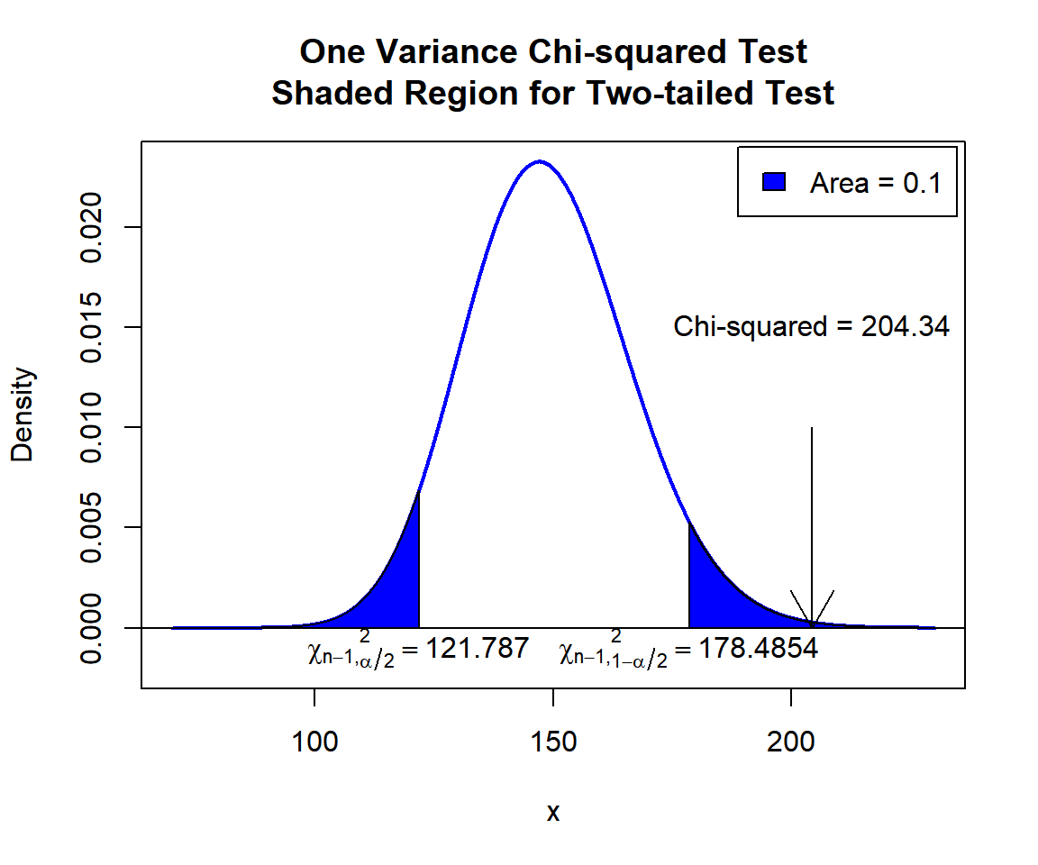

One Variance Chi-squared Test Shaded Region for Two-tailed Test in R

5 One-tailed One Variance Chi-squared Test in R

Right Tailed Test

For Petal.Length from the iris data, the sample variance is $s^2 = 3.1162779$ (var(iris$Petal.Length)).

For the following null hypothesis $H_0$, and alternative hypothesis $H_1$, with the level of significance $\alpha=0.2$.

$H_0:$ the population variance is equal to 2.5 ($\sigma^2 = 2.5$).

$H_1:$ the population variance is greater than 2.5 ($\sigma^2 > 2.5$, hence one-sided).

Because the level of significance is $\alpha=0.2$, the level of confidence is $1 - \alpha = 0.8$.

VarTest(iris$Petal.Length,
        sigma.squared = 2.5,
        alternative = "greater",
        conf.level = 0.8)


    One Sample Chi-Square test on variance

data:  iris$Petal.Length
X-squared = 185.73, df = 149, p-value = 0.02209
alternative hypothesis: true variance is greater than 2.5
80 percent confidence interval:
 2.843382      Inf
sample estimates:
variance of x 
     3.116278

Interpretation:

P-value: With the p-value ($p = 0.02209$) being less than the level of significance 0.2, we reject the null hypothesis that the population variance is equal to 2.5.
$\chi^2$ T-statistic: With test statistics value ($\chi^2_{149} = 185.73$) being greater than the critical value, $\chi^2_{149, 1-\alpha}=\text{qchisq(0.8, 149)}$$=163.3004042$ (or in the shaded region), we reject the null hypothesis that the population variance is equal to 2.5.
Confidence Interval: With the null hypothesis population variance value ($\sigma^2 = 2.5$) being outside the confidence interval, $[2.843382,\infty)$, we reject the null hypothesis that the population variance is equal to 2.5.

x = seq(70, 230, 1/1000); y = dchisq(x, df=149)
plot(x, y, type = "l",
     xlim = c(70, 230), ylim = c(-0.002, min(max(y), 1)),
     main = "One Variance Chi-squared Test
Shaded Region for Right-tailed Test",
     xlab = "x", ylab = "Density",
     lwd = 2, col = "blue")
abline(h=0)
# Add shaded region and legend
point = qchisq(0.8, 149)
polygon(x = c(x[x >= point], 230, point),
        y = c(y[x >= point], 0, 0),
        col = "blue")
legend("topright", c("Area = 0.2"),
       fill = c("blue"), inset = 0.01)
# Add critical value and Chi-squared value
arrows(200, 0.01, 185.73, 0)
text(200, 0.011, "Chi-squared = 185.73")
text(163.3004, -0.001, expression(chi[n-1][','][1-alpha]^2==163.3004))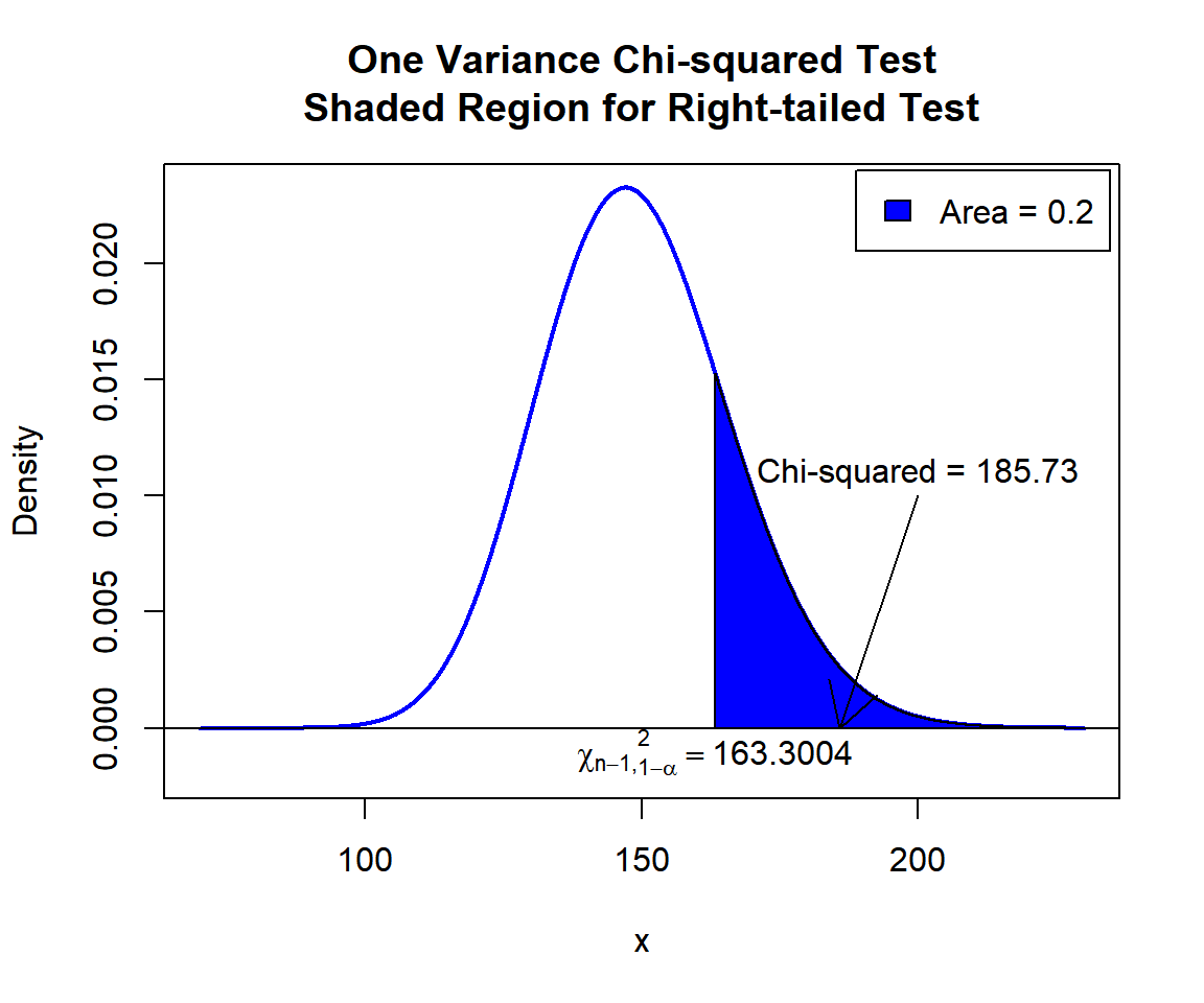

One Variance Chi-squared Test Shaded Region for Right-tailed Test in R

Left Tailed Test

For Petal.Width from the iris data, the sample variance is $s^2 = 0.5810063$ (var(iris$Petal.Width)).

For the following null hypothesis $H_0$, and alternative hypothesis $H_1$, with the level of significance $\alpha=0.1$.

$H_0:$ the population variance is equal to 0.6 ($\sigma^2 = 0.6$).

$H_1:$ the population variance is less than 0.6 ($\sigma^2 < 0.6$, hence one-sided).

Because the level of significance is $\alpha=0.1$, the level of confidence is $1 - \alpha = 0.9$.

VarTest(iris$Petal.Width,
        sigma.squared  = 0.6,
        alternative = "less",
        conf.level = 0.9)


    One Sample Chi-Square test on variance

data:  iris$Petal.Width
X-squared = 144.28, df = 149, p-value = 0.4062
alternative hypothesis: true variance is less than 0.6
90 percent confidence interval:
 0.0000000 0.6797833
sample estimates:
variance of x 
    0.5810063

Interpretation:

P-value: With the p-value ($p = 0.4062$) being greater than the level of significance 0.1, we fail to reject the null hypothesis that the population variance is equal to 0.6.
$\chi^2$ T-statistic: With test statistics value ($\chi^2_{149} = 144.28$) being greater than the critical value, $\chi^2_{149, \alpha}=\text{qchisq(0.1, 149)}$$=127.3493114$ (or not in the shaded region), we fail to reject the null hypothesis that the population variance is equal to 0.6.
Confidence Interval: With the null hypothesis population variance value ($\sigma^2_1 = 0.6$) being inside the confidence interval, $(0, 0.6797833]$, we fail reject the null hypothesis that the population variance is equal to 0.6.

x = seq(70, 230, 1/1000); y = dchisq(x, df=149)
plot(x, y, type = "l",
     xlim = c(70, 230), ylim = c(-0.002, min(max(y), 1)),
     main = "One Variance Chi-squared Test
Shaded Region for Left-tailed Test",
     xlab = "x", ylab = "Density",
     lwd = 2, col = "blue")
abline(h=0)
# Add shaded region and legend
point = qchisq(0.1, 149)
polygon(x = c(70, x[x <= point], point),
        y = c(0, y[x <= point], 0),
        col = "blue")
legend("topright", c("Area = 0.1"),
       fill = c("blue"), inset = 0.01)
# Add critical value and Chi-squared value
arrows(200, 0.01, 144.28, 0)
text(200, 0.011, "Chi-squared = 144.28")
text(127.3493, -0.001, expression(chi[n-1][','][alpha]^2==127.3493))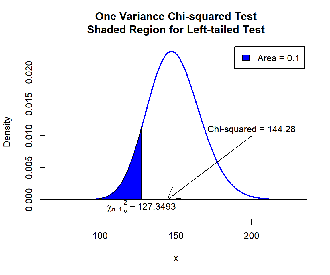

One Variance Chi-squared Test Shaded Region for Left-tailed Test in R

6 One Variance Chi-squared Test: Test Statistics, P-value & Degree of Freedom in R

Here for a one variance chi-squared test, we show how to get the test statistics (or chi-squared value), p-values, and degrees of freedom from the VarTest() function in R, or by written code.

data_ov = iris$Sepal.Width
var_object = VarTest(data_ov, sigma.squared = 0.2,
                   alternative = "two.sided",
                   conf.level = 0.95)
var_object


    One Sample Chi-Square test on variance

data:  data_ov
X-squared = 141.53, df = 149, p-value = 0.7471
alternative hypothesis: true variance is not equal to 0.2
95 percent confidence interval:
 0.1532698 0.2417372
sample estimates:
variance of x 
    0.1899794

To get the test statistic or chi-squared value:

\[\chi^2 = \frac{(n-1)s^2}{\sigma_0^2}.\]

var_object$statistic

X-squared 
 141.5347

# to remove name X-squared
unname(var_object$statistic)

[1] 141.5347

Same as:

sv = var(data_ov)
df = length(data_ov)-1
pv = 0.2
(df*sv)/pv

[1] 141.5347

To get the p-value:

Two-tailed: VarTest() uses a complex approach to calculate "two-sided" p-values which is illustrated below.

For an easier approach, for test statistics, $X^{U}$, when sample variance is greater than null hypothesis variance, and $X^{L}$, when sample variance is less than null hypothesis variance.

$Pvalue = 2*P(\chi^2_{df}>X^{U})$ or $Pvalue = 2*P(\chi^2_{df}<X^{L})$.

One-tailed: In the VarTest(), for right-tail, $Pvalue = P(\chi^2_{df}>X_{observed})$ or for left-tail, $Pvalue = P(\chi^2_{df}<X_{observed})$.

var_object$p.value

[1] 0.7471367

Same as:

Note that the p-value depends on the $\text{test statistics}$ ($\chi^2_{df} = 141.5347$), and $\text{degrees of freedom}$ (149). We also use the distribution functions pchisq() and dchisq() for the chi-squared distribution in R.

First, the density at $\chi^2_{149} = 141.5347$ is $0.0220607$ as dchisq(141.5347, 149) = 0.0220607. Similarly, on the other side of the mode $(df - 2 = 149-2 = 147)$, we have $\chi^2_{149} = 152.6042$ also having density as $0.0220607$, as dchisq(152.6042, 149) = 0.0220607.

Hence, the p-value for VarTest() is calculated as follows. The sum of the left tail region from the smaller value on the left side of the mode, and the right tail region from the higher value on the right side of the mode.

pchisq(141.5347, 149) + (1-pchisq(152.6042, 149))

[1] 0.7471385

Easier and alternate approach:

2*(pchisq(141.5347, 149))

[1] 0.688347

To get the degrees of freedom:

The degrees of freedom are $\text{df}=149$.

var_object$parameter

 df 
149

# to remove name df
unname(var_object$parameter)

[1] 149

Same as:

length(data_ov)-1

[1] 149

7 One Variance Chi-squared Test: Estimate & Confidence Interval in R

Here for a one variance chi-squared test, we show how to get the sample variances and confidence interval from the VarTest() function in R, or by written code.

data_ov = iris$Sepal.Width
var_object = VarTest(data_ov, sigma.squared = 0.2,
                   alternative = "two.sided",
                   conf.level = 0.9)
var_object


    One Sample Chi-Square test on variance

data:  data_ov
X-squared = 141.53, df = 149, p-value = 0.7471
alternative hypothesis: true variance is not equal to 0.2
90 percent confidence interval:
 0.1585953 0.2324298
sample estimates:
variance of x 
    0.1899794

To get the point estimate or sample variance:

\[s^2 = \frac{1}{n-1}\sum_{i=1}^n (x_i-\bar x)^2, \quad \bar x = \frac{1}{n}\sum_{i=1}^n x_i.\]

var_object$estimate

variance of x 
    0.1899794

# to remove name variance of x
unname(var_object$estimate)

[1] 0.1899794

Same as:

var(data_ov)

Or:

sum((data_ov-mean(data_ov))^2)/(length(data_ov)-1)

[1] 0.1899794

To get the confidence interval for $\sigma^2$:

For two-tailed:

\[CI = \left[\frac{(n-1)s^2}{\chi^2_{df, 1-\alpha/2}} \;,\; \frac{(n-1)s^2}{\chi^2_{df, \alpha/2}} \right].\]

For right one-tailed:

\[CI = \left[\frac{(n-1)s^2}{\chi^2_{df, 1-\alpha}} \;,\; \infty \right).\]

For left one-tailed:

\[CI = \left(0 \;,\; \frac{(n-1)s^2}{\chi^2_{df, \alpha}} \right].\]

var_object$conf.int

[1] 0.1585953 0.2324298
attr(,"conf.level")
[1] 0.9

# to remove attr conf.int
var_object$conf.int[1:2]

[1] 0.1585953 0.2324298

Same as:

sv = var(data_ov)
df = length(data_ov)-1; alpha = 0.1
xl = qchisq(1-alpha/2, df)
l = (df*sv)/xl
xu = qchisq(alpha/2, df)
u = (df*sv)/xu
c(l, u)

[1] 0.1585953 0.2324298

One tailed example:

sv = var(data_ov)
df = length(data_ov)-1; alpha = 0.1
#Right Tail
xl = qchisq(alpha, df)
l = (df*sv)/xl
c(l, Inf)
#Left Tail
xu = qchisq(1-alpha, df)
u = (df*sv)/xu
c(0, u)

Question	Is the variance equal to \(\sigma_0\)?	Is the variance greater than \(\sigma_0\)?	Is the variance less than \(\sigma_0\)?
Form of Test	Two-tailed	Right-tailed test	Left-tailed test
Null Hypothesis, \(H_0\)	\(\sigma = \sigma_0\)	\(\sigma = \sigma_0\)	\(\sigma = \sigma_0\)
Alternate Hypothesis, \(H_1\)	\(\sigma \neq \sigma_0\)	\(\sigma > \sigma_0\)	\(\sigma < \sigma_0\)

One Variance Chi-squared Tests in R

Install and Load the "DescTools" Package:

Sample Steps to Run a One Variance Chi-squared Test:

Creating a One Variance Chi-squared Test Object:

1 Test Statistic for One Variance Chi-squared Test in R

2 Simple One Variance Chi-squared Test in R

Interpretation:

3 One Variance Chi-squared Test Critical Value in R

4 Two-tailed One Variance Chi-squared Test in R

Interpretation:

5 One-tailed One Variance Chi-squared Test in R

Right Tailed Test

Interpretation:

Left Tailed Test

Interpretation:

6 One Variance Chi-squared Test: Test Statistics, P-value & Degree of Freedom in R

To get the test statistic or chi-squared value:

To get the p-value:

To get the degrees of freedom:

7 One Variance Chi-squared Test: Estimate & Confidence Interval in R

To get the point estimate or sample variance:

To get the confidence interval for \(\sigma^2\):