Negative Binomial Distributions in R
- 1 Table of Negative Binomial Distribution Functions in R
- 2 Plot of Negative Binomial Distributions in R
- 3 Examples for Setting Parameters for Negative Binomial Distributions in R
- 4 rnbinom(): Random Sampling from Negative Binomial Distributions in R
- 5 dnbinom(): Probability Mass Function for Negative Binomial Distributions in R
- 6 pnbinom(): Cumulative Distribution Function for Negative Binomial Distributions in R
- 7 qnbinom(): Derive Quantile for Negative Binomial Distributions in R
Here, we discuss negative binomial distribution functions in R, plots, parameter setting, random sampling, mass function, cumulative distribution and quantiles.
The negative binomial distribution for the number of failures before reaching \(n\) successes in a sequence of independent and identically distributed Bernoulli trials, with parameters \(\tt{size}=n\), and \(\tt{probability\:of\:success}=p\) has probability mass function (pmf) formula as:
\[\begin{align} P(X=x)&=\binom{x+n-1}{n-1} p^n(1-p)^x \\ & = \binom{x+n-1}{x} p^n(1-p)^x \\ & = \frac{(x+n-1)!}{x!(n-1)!} p^n(1-p)^x,\end{align}\] for \(x \in \{0, 1, 2, \ldots\}\) number of failures,
where \(n > 0\) is the fixed number of successes to be reached,
\(p \in (0,1]\) is the probability of success in each trial,
the \(\tt{binomial\; coefficient}\) \(\binom{a}{b}\) equals \(\frac{a!}{b!(a-b)!}\),
and \(a!\), the \(\tt{factorial\; operator}\), equals \(a\times(a-1)\times(a-2)\times\cdots\times 1\).
The mean is \(\frac{n(1-p)}{p}\), and the variance is \(\frac{n(1-p)}{p^2}\).
See also probability distributions and plots and charts.
1 Table of Negative Binomial Distribution Functions in R
The table below shows the functions for negative binomial distributions in R.
| Function | Usage |
| rnbinom(n, size, prob, mu) | Simulate a random sample with \(n\) observations |
| dnbinom(x, size, prob, mu) | Calculate the probability mass at the point \(x\) |
| pnbinom(q, size, prob, mu) | Calculate the cumulative distribution at the point \(q\) |
| qnbinom(p, size, prob, mu) | Calculate the quantile value associated with \(p\) |
The examples here are based on the \(\tt{size}\) and \(\tt{prob}\) parameters in the pmf above, as only one of the "prob" and "mu" arguments can be specified at a time. Hence, the "mu" argument (for \(\tt{mean}\)) is excluded in the examples below.
However, to use the \(\tt{mean}\) parameter, you can set the argument to the mean value of the distribution. For example:
[1] 0.1180456Which (since \(\tt{prob = size/(size + mu)}\)) is equivalent to:
[1] 0.11804562 Plot of Negative Binomial Distributions in R
Single distribution:
Below is a plot of the negative binomial distribution function with \(\tt{size}=10\), and \(\tt{probability\:of\:success}=0.4\).
x = 0:40; y = dnbinom(x, 10, 0.4)
plot(x, y, type = "h",
     xlim = c(0, 40), ylim = c(0, max(y)),
     main = "Probability Mass Function of
Negative Binomial Distribution (10, 0.4)",
     xlab = "x", ylab = "Mass",
     col = "blue")
# Add legend
legend("topright", "size = 10, prob = 0.4",
       fill = "blue",
       bty = "n")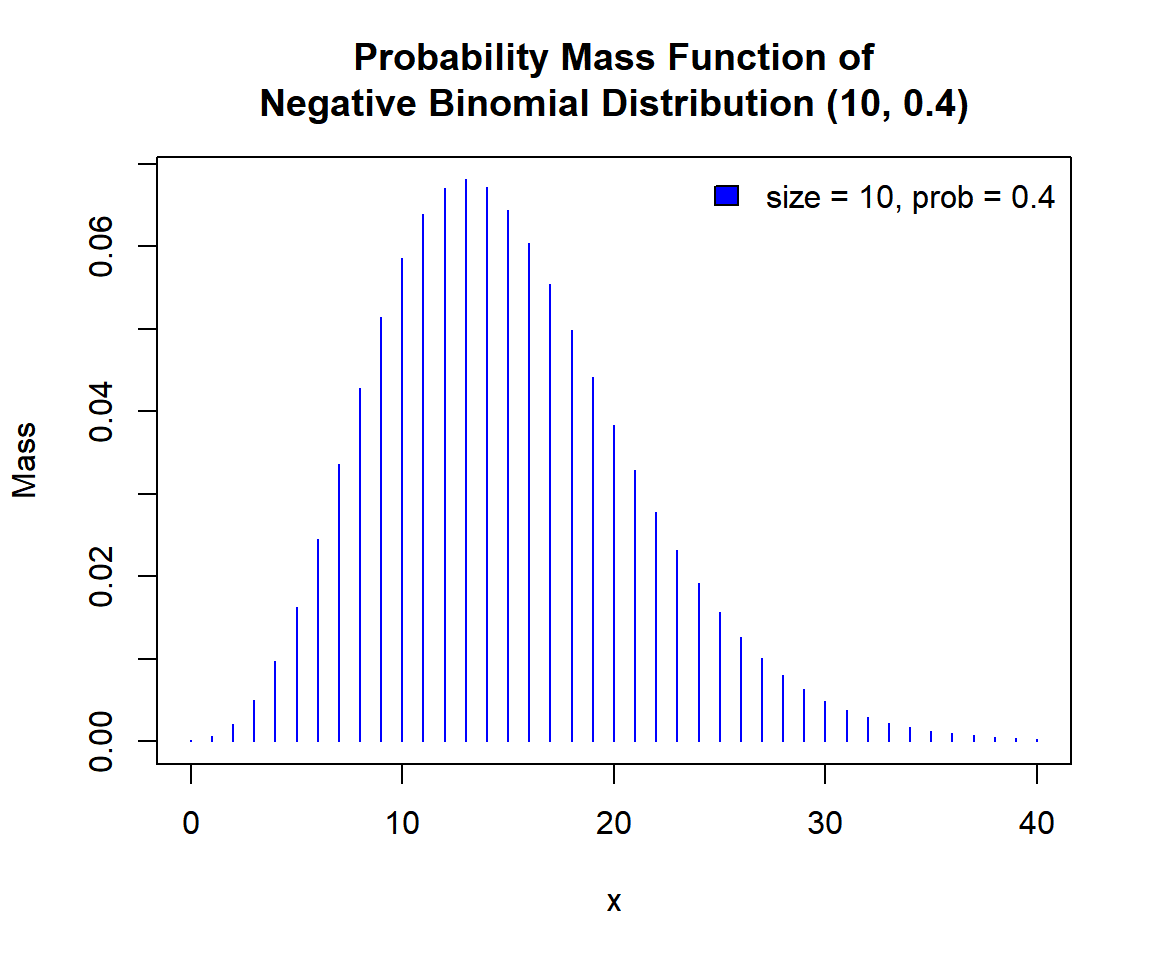
Probability Mass Function (PMF) of a Negative Binomial Distribution in R
Multiple distributions:
Below is a plot of multiple negative binomial distribution functions in one graph.
x1 = 0:15; y1 = dnbinom(x1, 6, 0.7)
x2 = 0:30; y2 = dnbinom(x2, 6, 0.35)
x3 = 0:20; y3 = dnbinom(x3, 9, 0.7)
plot(x1, y1,
     xlim = c(0, 30), ylim = range(c(y1, y2, y3)),
     main = "Probability Mass Functions of
Negative Binomial Distributions",
     xlab = "x", ylab = "Mass",
     col = "blue")
points(x2, y2, col = "red")
points(x3, y3, col = "green")
# Add legend
legend("topright", c("size = 6, prob = 0.7",
                    "size = 6, prob = 0.35",
                    "size = 9, prob = 0.7"),
       fill = c("blue", "red", "green"),
       bty = "n")
# Add lines
for(i in 1:15){
  segments(x1[i], dnbinom(x1[i], 6, 0.7),
           x1[i+1], dnbinom(x1[i+1], 6, 0.7),
           col = "blue")}
for(i in 1:30){
  segments(x2[i], dnbinom(x2[i], 6, 0.35),
           x2[i+1], dnbinom(x2[i+1], 6, 0.35),
           col = "red")}
for(i in 1:20){
  segments(x3[i], dnbinom(x3[i], 9, 0.7),
           x3[i+1], dnbinom(x3[i+1], 9, 0.7),
           col = "green")}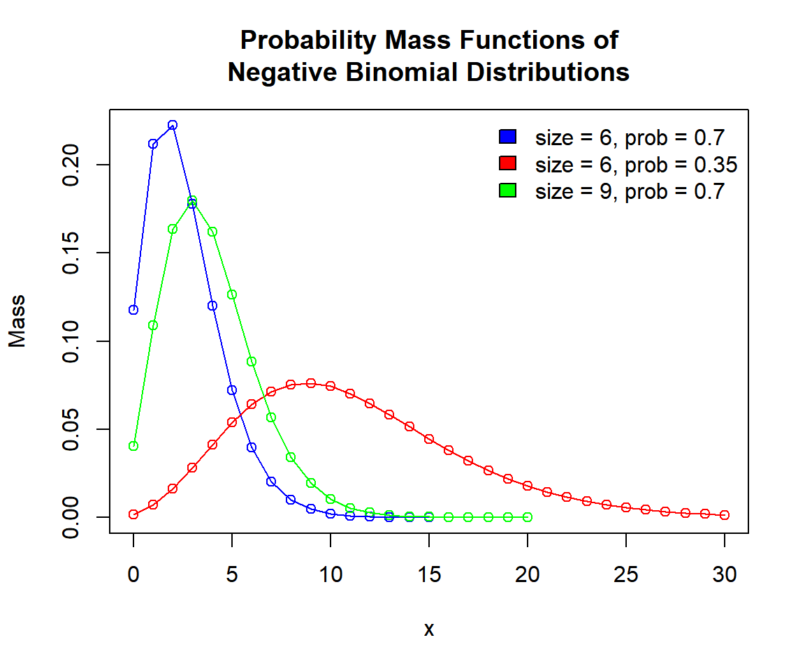
Probability Mass Functions (PMFs) of Negative Binomial Distributions in R
3 Examples for Setting Parameters for Negative Binomial Distributions in R
To set the parameters for the negative binomial distribution function, with \(\tt{size}=12\) and \(\tt{probability\:of\:success}=0.35\).
For example, for pnbinom(), the following are the
same:
# The order of 12 and 0.35 matters here as the parameter names are not used.
# The first number 12 is size, and 0.35 is prob.
pnbinom(8, 12, 0.35)
[1] 0.01957936[1] 0.01957936[1] 0.019579364 rnbinom(): Random Sampling from Negative Binomial Distributions in R
Sample 650 observations from the negative binomial distribution with \(\tt{size}=7\) and \(\tt{probability\:of\:success}=0.2\):
set.seed(12) # Line allows replication (use any number).
sample = rnbinom(650, 7, 0.2)
hist(sample,
     main = "Histogram of 650 Observations from
Negative Binomial Distribution with Size = 7 and Prob = 0.2",
     xlab = "x",
     col = "lightblue", border = "white")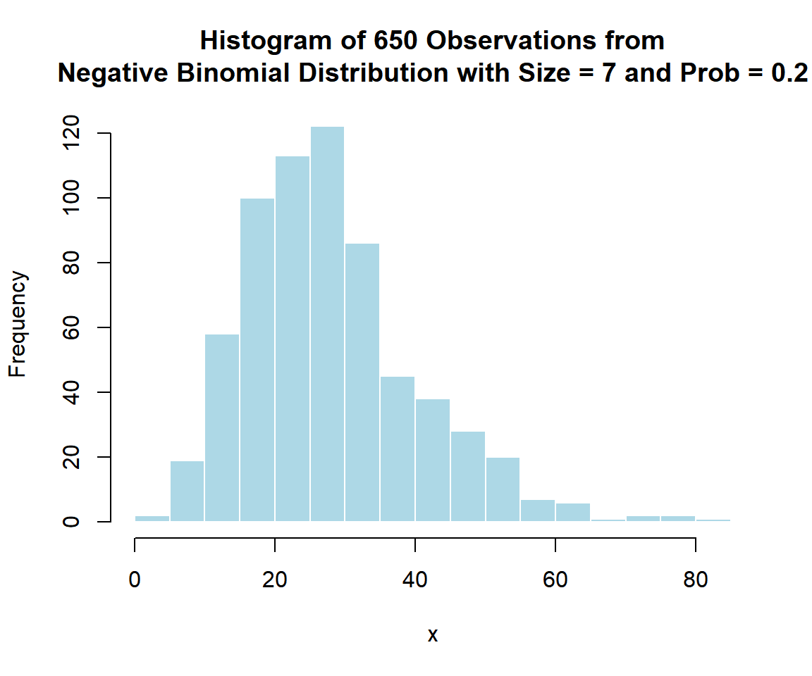
Histogram of Negative Binomial Distribution (7, 0.2) Random Sample in R
5 dnbinom(): Probability Mass Function for Negative Binomial Distributions in R
Calculate the mass at \(x = 2\), in the negative binomial distribution with \(\tt{size}=5\) and \(\tt{probability\:of\:success}=0.7\):
[1] 0.2268945x = 0:10; y = dnbinom(x, 5, 0.7)
plot(x, y,
xlim = c(0, 10), ylim = c(0, max(y)),
main = "Probability Mass Function of
Negative Binomial Distribution with Size = 5 and Prob = 0.7",
xlab = "x", ylab = "Mass",
col = "blue")
# Add lines
segments(2, -1, 2, 0.2268945)
segments(-1, 0.2268945, 2, 0.2268945)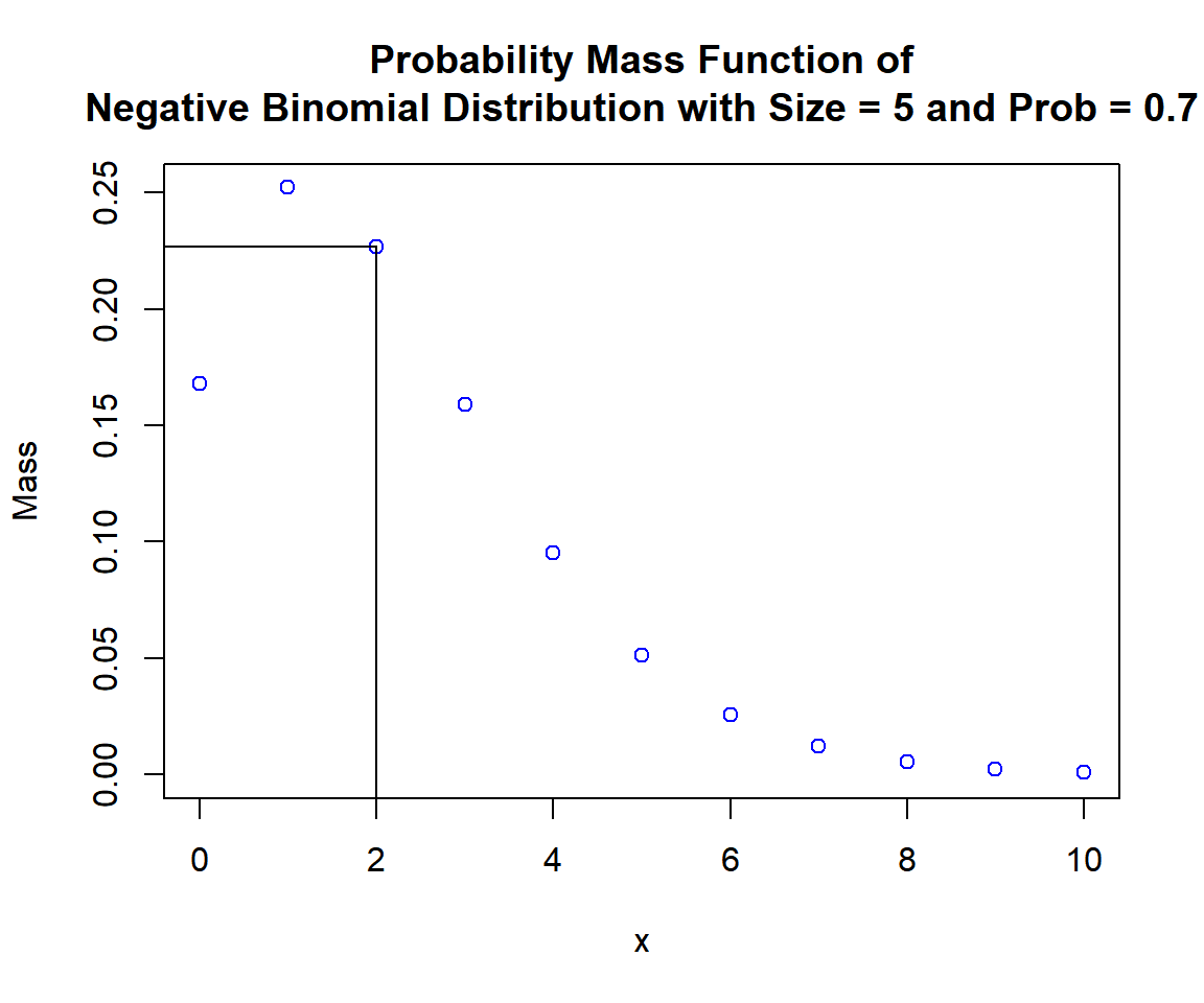
Probability Mass Function (PMF) of Negative Binomial Distribution (5, 0.7) in R
6 pnbinom(): Cumulative Distribution Function for Negative Binomial Distributions in R
Calculate the cumulative distribution at \(x = 8\), in the negative binomial distribution with \(\tt{size}=6\) and \(\tt{probability\:of\:success}=0.5\). That is, \(P(X \le 8)\):
[1] 0.7880249x = 0:15; y = pnbinom(x, 6, 0.5)
plot(x, y,
xlim = c(0, 15), ylim = c(0, 1),
main = "Cumulative Distribution Function of
Negative Binomial Distribution with Size = 6 and Prob = 0.5",
xlab = "x", ylab = "Cumulative Distribution",
col = "blue")
# Add lines
for(i in 1:15){
segments(x[i], pnbinom(x[i], 6, 0.5),
x[i] + 1, pnbinom(x[i], 6, 0.5),
col = "blue")
}
segments(8, -1, 8, 0.7880249)
segments(-1, 0.7880249, 8, 0.7880249)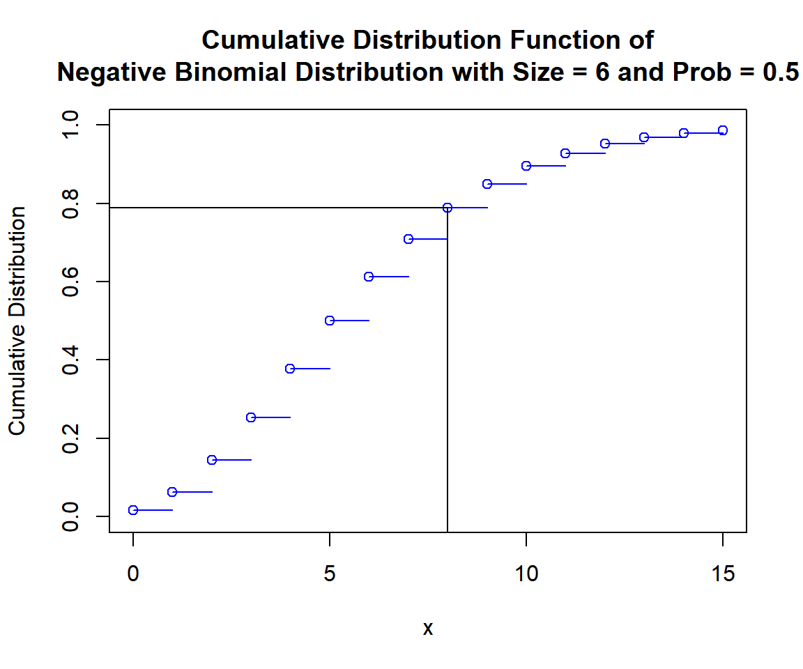
Cumulative Distribution Function (CDF) of Negative Binomial Distribution (6, 0.5) in R
For upper tail, at \(x = 8\), that is, \(P(X > 8) = 1 - P(X \le 8)\), set the "lower.tail" argument:
[1] 0.21197517 qnbinom(): Derive Quantile for Negative Binomial Distributions in R
Derive the quantile for \(p = 0.8\), in the negative binomial distribution with \(\tt{size}=7\) and \(\tt{probability\:of\:success}=0.6\). That is, the \(\tt{smallest}\) \(x\) such that, \(P(X\le x) \ge 0.8\):
[1] 7x = 0:15; y = pnbinom(x, 7, 0.6)
plot(x, y,
xlim = c(0, 15), ylim = c(0, 1),
main = "Cumulative Distribution Function of
Negative Binomial Distribution with Size = 7 and Prob = 0.6",
xlab = "x", ylab = "Cumulative Distribution",
col = "blue")
# Add lines
for(i in 1:15){
segments(x[i], pnbinom(x[i], 7, 0.6),
x[i] + 1, pnbinom(x[i], 7, 0.6),
col = "blue")
}
segments(7, -1, 7, 0.8)
segments(-1, 0.8, 7, 0.8)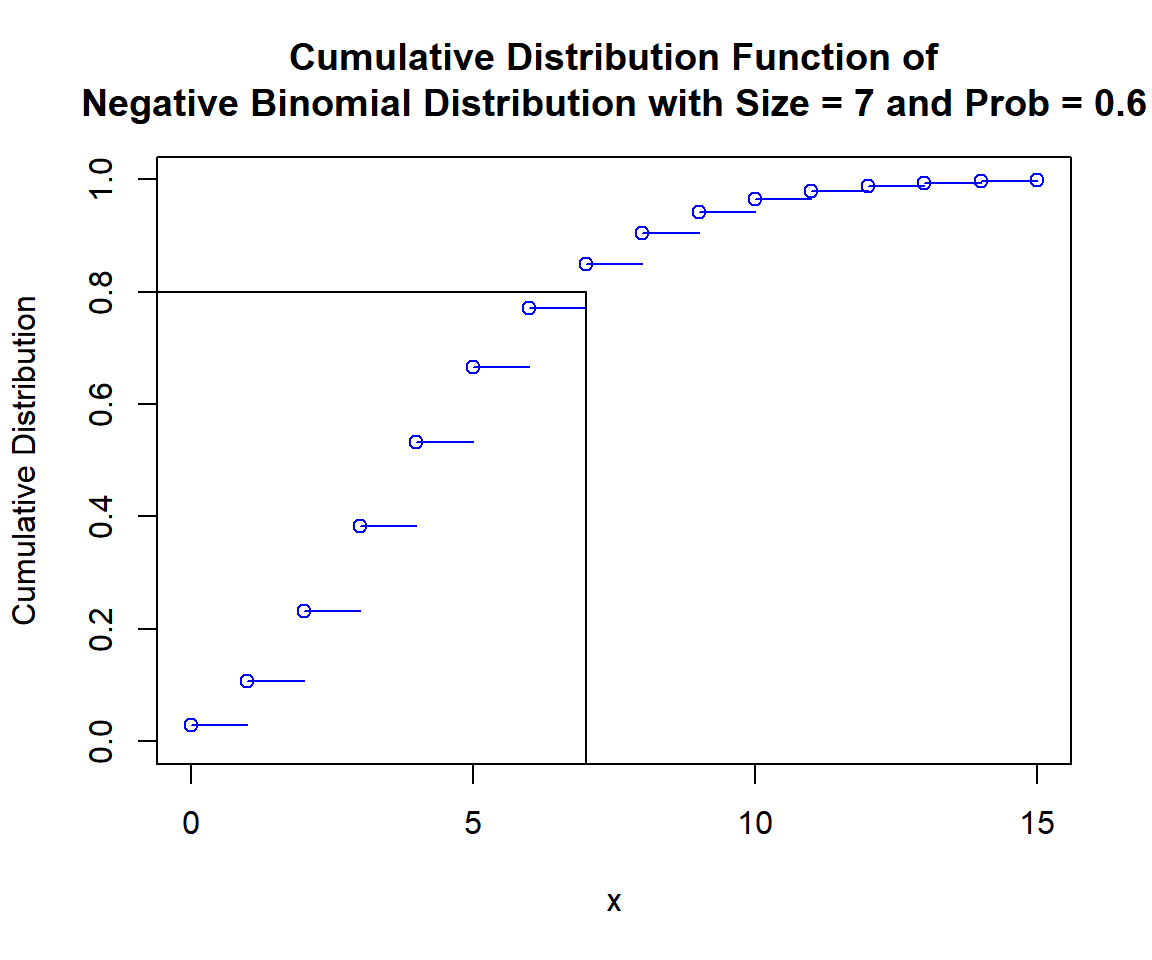
Cumulative Distribution Function (CDF) of Negative Binomial Distribution (7, 0.6) in R
For upper tail, for \(p = 0.2\), that is, the \(\tt{smallest}\) \(x\) such that, \(P(X > x) < 0.2\):
Note: \(P(X > x) = 1-P(X \le x)\).
[1] 7The feedback form is a Google form but it does not collect any personal information.
Please click on the link below to go to the Google form.
Thank You!
Go to Feedback Form
Copyright © 2020 - 2026. All Rights Reserved by Stats Codes