1 Table of Lognormal Distribution Functions in R
2 Plot of Lognormal Distributions in R
3 Examples for Setting Parameters for Lognormal Distributions in R
4 rlnorm(): Random Sampling from Lognormal Distributions in R
5 dlnorm(): Probability Density Function for Lognormal Distributions in R
6 plnorm(): Cumulative Distribution Function for Lognormal Distributions in R
7 qlnorm(): Derive Quantile for Lognormal Distributions in R

Here, we discuss lognormal distribution functions in R, plots, parameter setting, random sampling, density, cumulative distribution and quantiles.

The lognormal distribution with parameters \(\tt{meanlog}=\mu\), and \(\tt{sdlog}=\sigma\) has probability density function (pdf) formula as:

\[f(x)=\frac 1 {x\sigma\sqrt{2\pi}}\ e^{-{\frac {1}{2}}\left({\frac {\ln(x)-\mu }{\sigma }}\right)^{2}},\] for \(x \in (0, +\infty)\),

where \(\mu \in \mathbb {R}\), and \(\sigma>0\).

\(e\) is \(\tt{Euler's\;number}\) with \(e \approx 2.71828\), and \(\pi\approx 3.14159\).

The mean is \(e^{\left(\mu+\frac{\sigma^2}{2}\right)}\), and variance is \(e^{(2\mu+\sigma^2)}*[e^{\sigma^2}-1]\).

Note: If \(X \sim\tt{Lognorm} (\mu, \sigma)\), then \(\tt{\ln(X)} \sim \tt{Normal} (\mu, \sigma)\); or if \(X \sim \tt{Normal} (\mu, \sigma)\), then \(\tt{\exp(X)} \sim\tt{Lognorm} (\mu, \sigma)\).

1 Table of Lognormal Distribution Functions in R

The table below shows the functions for lognormal distributions in R.

Table of Lognormal Distribution Functions in R
Function	Usage
rlnorm(n, meanlog=0, sdlog=1)	Simulate a random sample with \(n\) observations
dlnorm(x, meanlog=0, sdlog=1)	Calculate the probability density at the point \(x\)
plnorm(q, meanlog=0, sdlog=1)	Calculate the cumulative distribution at the point \(q\)
qlnorm(p, meanlog=0, sdlog=1)	Calculate the quantile value associated with \(p\)

2 Plot of Lognormal Distributions in R

Single distribution:

Below is a plot of the lognormal distribution function with \(\tt{meanlog}=2\) and \(\tt{sdlog}=0.6\).

x = seq(0, 35, 1/1000); y = dlnorm(x, 2, 0.6)
plot(x, y, type = "l",
     xlim = c(0, 35), ylim = c(0, max(y)),
     main = "Probability Density Function of
Lognormal Distribution (2, 0.6)",
     xlab = "x", ylab = "Density",
     lwd = 2, col = "blue")
# Add legend
legend("topright", "meanlog = 2, sdlog = 0.6",
       lwd = 2,
       col = "blue",
       bty = "n")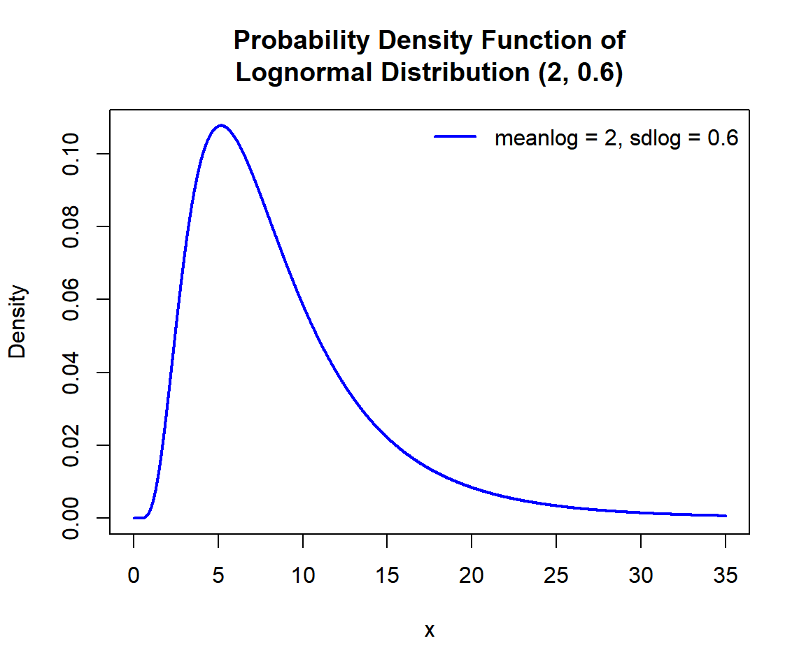

Probability Density Function (PDF) of a Lognormal Distribution in R

Multiple distributions:

Below is a plot of multiple lognormal distribution functions in one graph.

x1 = seq(0, 10, 1/1000); y1 = dlnorm(x1, 0, 1)
x2 = seq(0, 10, 1/1000); y2 = dlnorm(x2, 0.5, 0.75)
x3 = seq(0, 10, 1/1000); y3 = dlnorm(x3, -0.25, 1.2)
plot(x1, y1, type = "l",
     xlim = c(0, 10), ylim = range(c(y1, y2, y3)),
     main = "Probability Density Functions of Lognormal Distributions",
     xlab = "x", ylab = "Density",
     lwd = 2, col = "blue")
points(x2, y2, type = "l", lwd = 2, col = "red")
points(x3, y3, type = "l", lwd = 2, col = "green")
# Add legend
legend("topright", c("meanlog = 0,       sdlog = 1",
                    "meanlog = 0.5,    sdlog = 0.75",
                    "meanlog = -0.25, sdlog = 1.2"),
       lwd = c(2, 2, 2),
       col = c("blue", "red", "green"),
       bty = "n")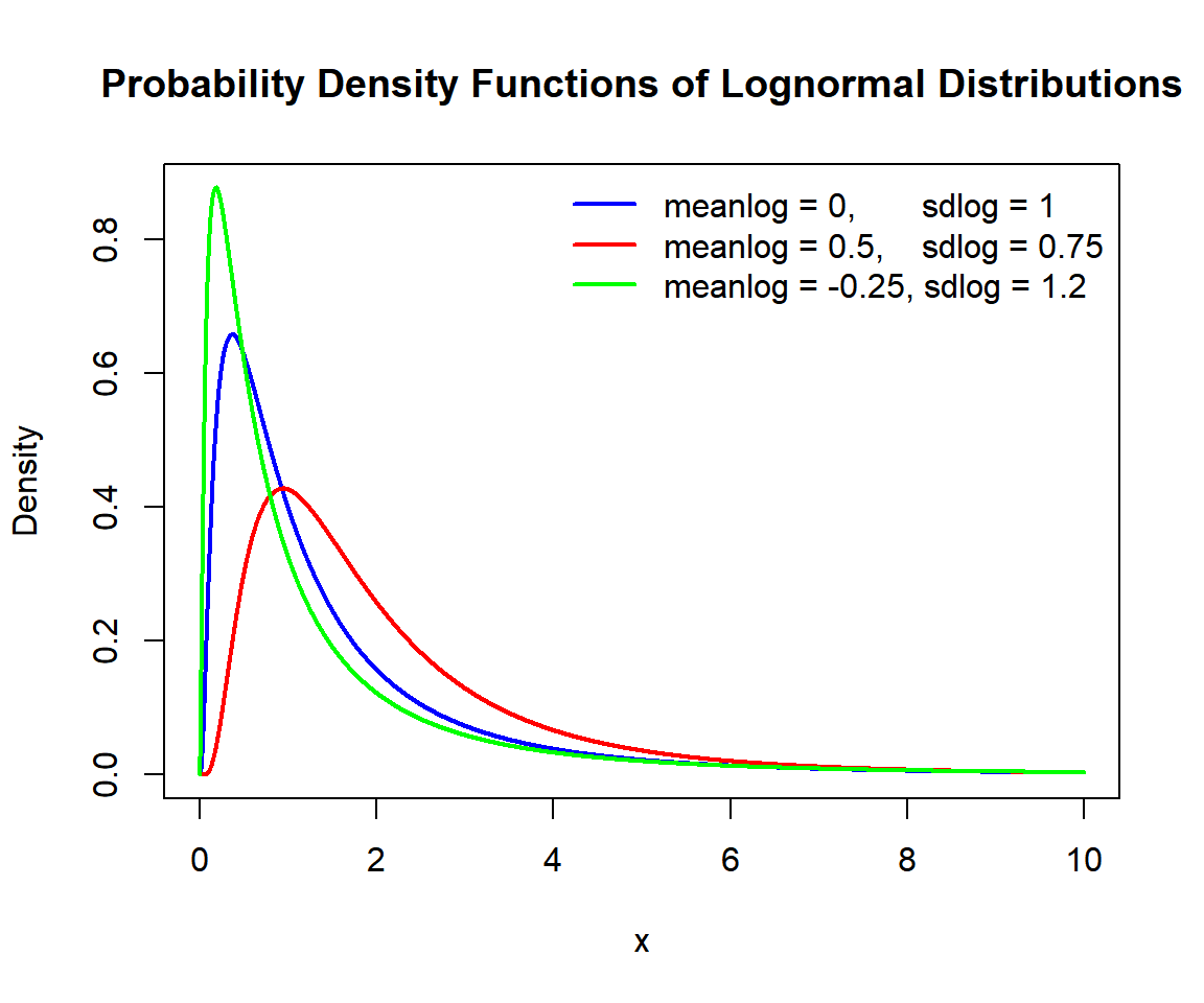

Probability Density Functions (PDFs) of Lognormal Distributions in R

3 Examples for Setting Parameters for Lognormal Distributions in R

In the lognormal distribution functions, parameters are pre-specified as \(\tt{meanlog}=0\) and \(\tt{sdlog}=1\), hence they do not need to be specified, unless they are to be set to different values.

For example, for dlnorm(), the following are the same:

# The order of 0 and 1 matters here as the parameter names are not used.
# The first number 0 is meanlog, and 1 is sdlog.
dlnorm(2); dlnorm(2, 0); dlnorm(2, 0, 1)

[1] 0.156874

[1] 0.156874

[1] 0.156874

# Or:
dlnorm(2, meanlog = 0, sdlog = 1)

[1] 0.156874

# Or:
dlnorm(2, sdlog = 1, meanlog = 0)

[1] 0.156874

4 rlnorm(): Random Sampling from Lognormal Distributions in R

Sample 1500 observations from the lognormal distribution with \(\tt{meanlog} = 1.8\) and \(\tt{sdlog} = 0.5\):

rlnorm(1500, 1.8, 0.5)

set.seed(123) # Line allows replication (use any number).
sample = rlnorm(1500, 1.8, 0.5)
hist(sample,
     main = "Histogram of 1500 Observations from Lognormal Distribution
with Meanlog = 1.8 and SDlog = 0.5",
     xlab = "x",
     col = "deepskyblue", border = "white")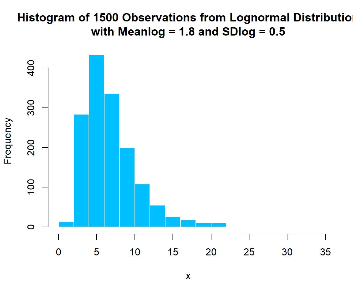

Histogram of Lognormal Distribution (1.8, 0.5) Random Sample in R

5 dlnorm(): Probability Density Function for Lognormal Distributions in R

Calculate the density at \(x = 4\), in the lognormal distribution with \(\tt{meanlog} = 0.75\) and \(\tt{sdlog} = 0.6\):

dlnorm(4, 0.75, 0.6)

[1] 0.09472973

x = seq(0, 12, 1/1000); y = dlnorm(x, 0.75, 0.6)
plot(x, y, type = "l",
     xlim = c(0, 12), ylim = c(0, max(y)),
     main = "Probability Density Function of Lognormal Distribution
with Mean = 0.75 and SDlog = 0.6",
     xlab = "x", ylab = "Density",
     lwd = 2, col = "blue")
# Add lines
segments(4, -1, 4, 0.09472973)
segments(-1, 0.09472973, 4, 0.09472973)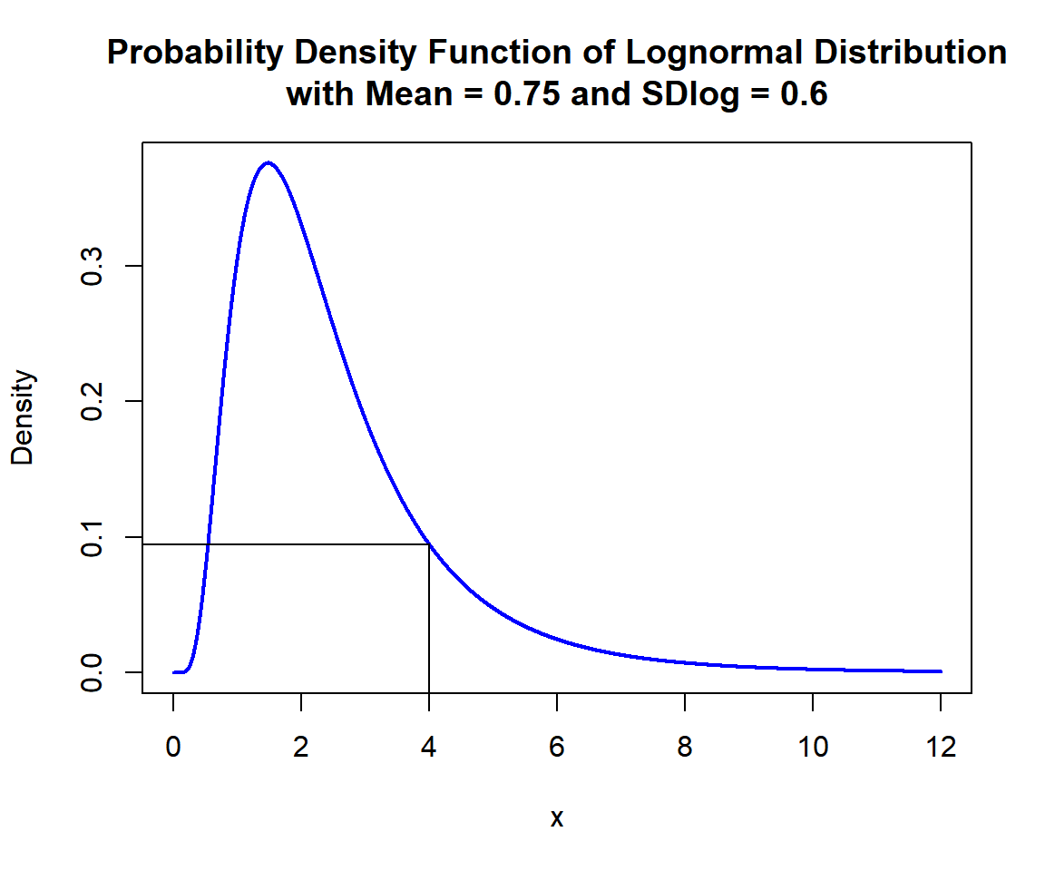

Probability Density Function (PDF) of Lognormal Distribution (0.75, 0.6) in R

6 plnorm(): Cumulative Distribution Function for Lognormal Distributions in R

Calculate the cumulative distribution at \(x = 2.5\), in the lognormal distribution with \(\tt{meanlog} = 0.8\) and \(\tt{sdlog} = 0.5\). That is, \(P(X \le 2.5)\):

plnorm(2.5, 0.8, 0.5)

[1] 0.5919568

x = seq(0, 10, 1/1000); y = plnorm(x, 0.8, 0.5)
plot(x, y, type = "l",
     xlim = c(0, 10), ylim = c(0,1),
     main = "Cumulative Distribution Function of Lognormal Distribution
with Meanlog = 0.8 and SDlog = 0.5",
     xlab = "x", ylab = "Cumulative Distribution",
     lwd = 2, col = "blue")
# Add lines
segments(2.5, -1, 2.5, 0.5919568)
segments(-1, 0.5919568, 2.5, 0.5919568)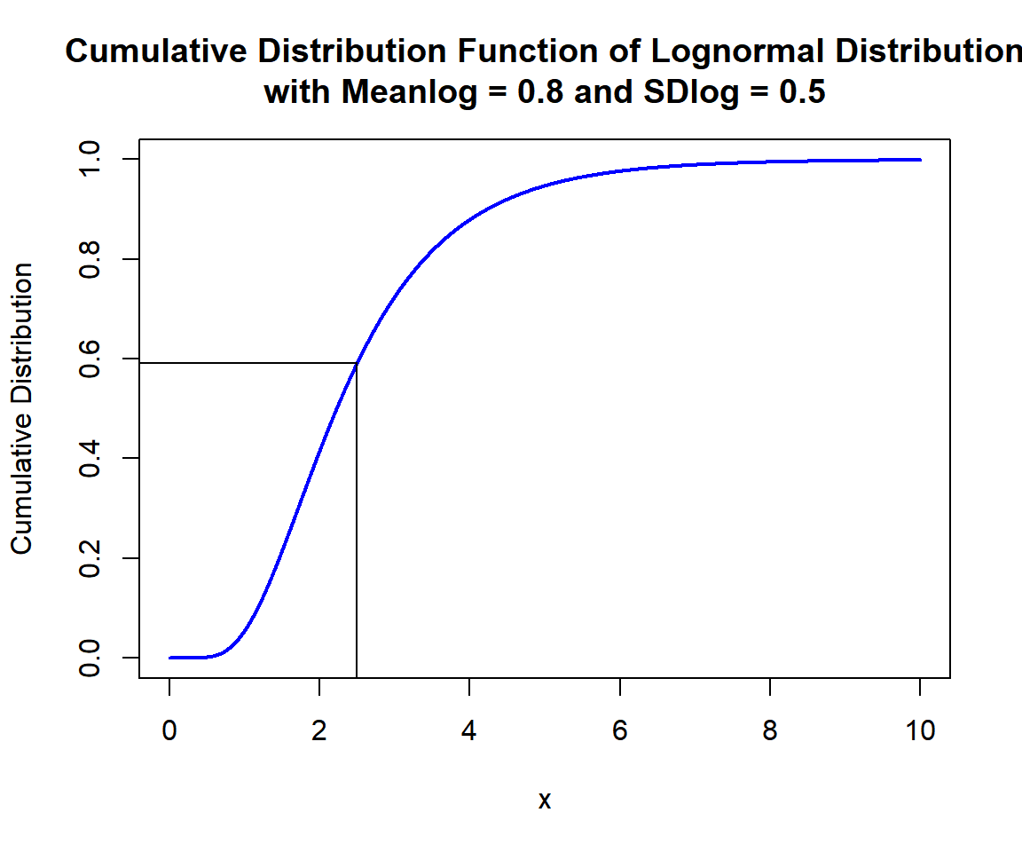

Cumulative Distribution Function (CDF) of Lognormal Distribution (0.8, 0.5) in R

x = seq(0, 10, 1/1000); y = dlnorm(x, 0.8, 0.5)
plot(x, y, type = "l",
     xlim = c(0, 10), ylim = c(0, max(y)),
     main = "Probability Density Function of Lognormal Distribution
with Meanlog = 0.8 and SDlog = 0.5",
     xlab = "x", ylab = "Density",
     lwd = 2, col = "blue")
# Add shaded region and legend
point = 2.5
polygon(x = c(x[x <= point], point),
        y = c(y[x <= point], 0),
        col = "limegreen")
legend("topright", c("Area = 0.5919568"),
       fill = c("limegreen"),
       inset = 0.01)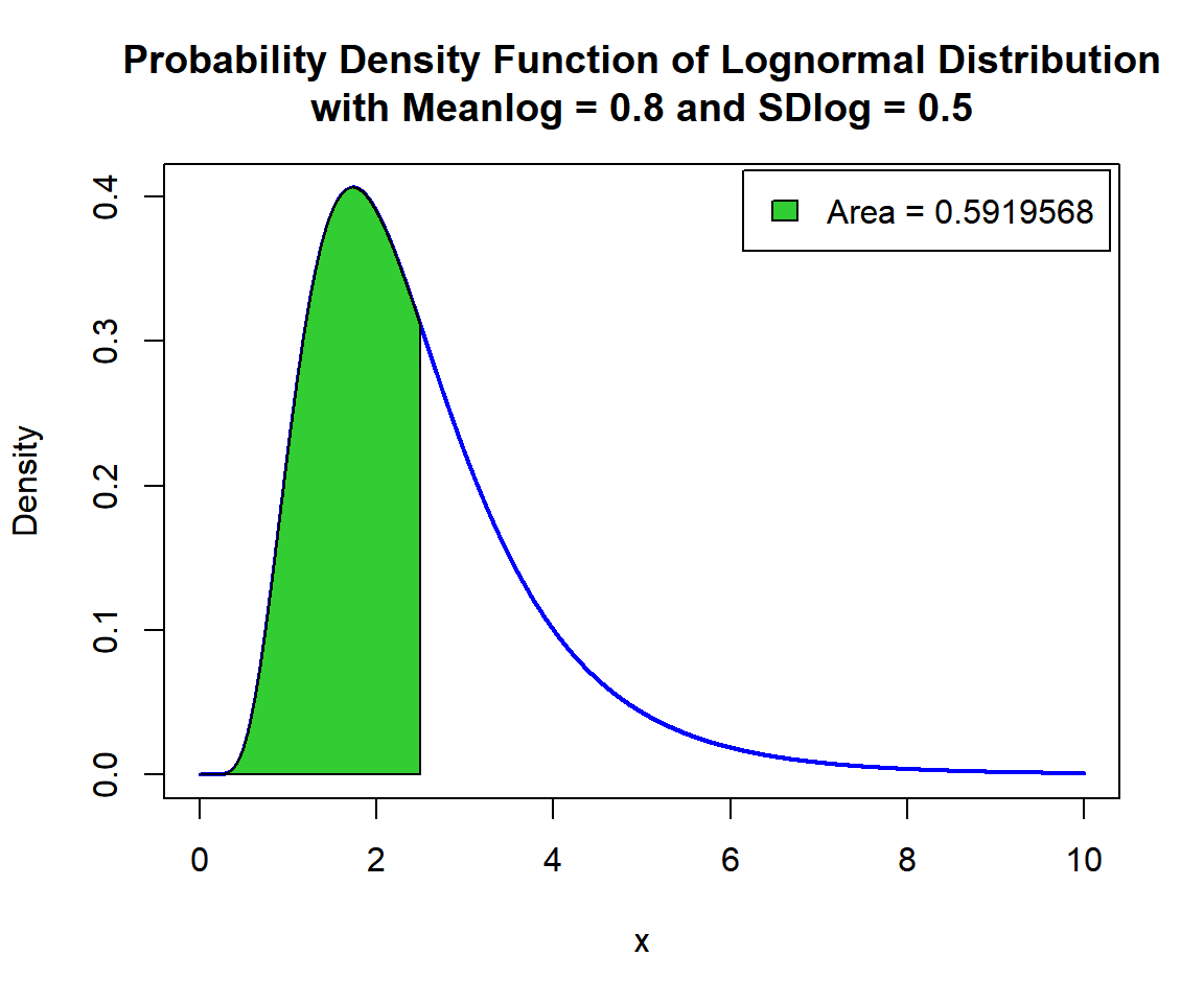

Shaded Probability Density Function (PDF) of Lognormal Distribution (0.8, 0.5) in R

For upper tail, at \(x = 2.5\), that is, \(P(X \ge 2.5) = 1 - P(X \le 2.5)\), set the "lower.tail" argument:

plnorm(2.5, 0.8, 0.5, lower.tail = FALSE)

[1] 0.4080432

x = seq(0, 10, 1/1000); y = dlnorm(x, 0.8, 0.5)
plot(x, y, type = "l",
     xlim = c(0, 10), ylim = c(0, max(y)),
     main = "Shaded Upper Region: Probability Density Function of
Lognormal Distribution with Meanlog = 0.8 and SDlog = 0.5",
     xlab = "x", ylab = "Density",
     lwd = 2, col = "blue")
# Add shaded region and legend
point = 2.5
polygon(x = c(point, x[x >= point]),
        y = c(0, y[x >= point]),
        col = "limegreen")
legend("topright", c("Area = 0.4080432"),
       fill = c("limegreen"),
       inset = 0.01)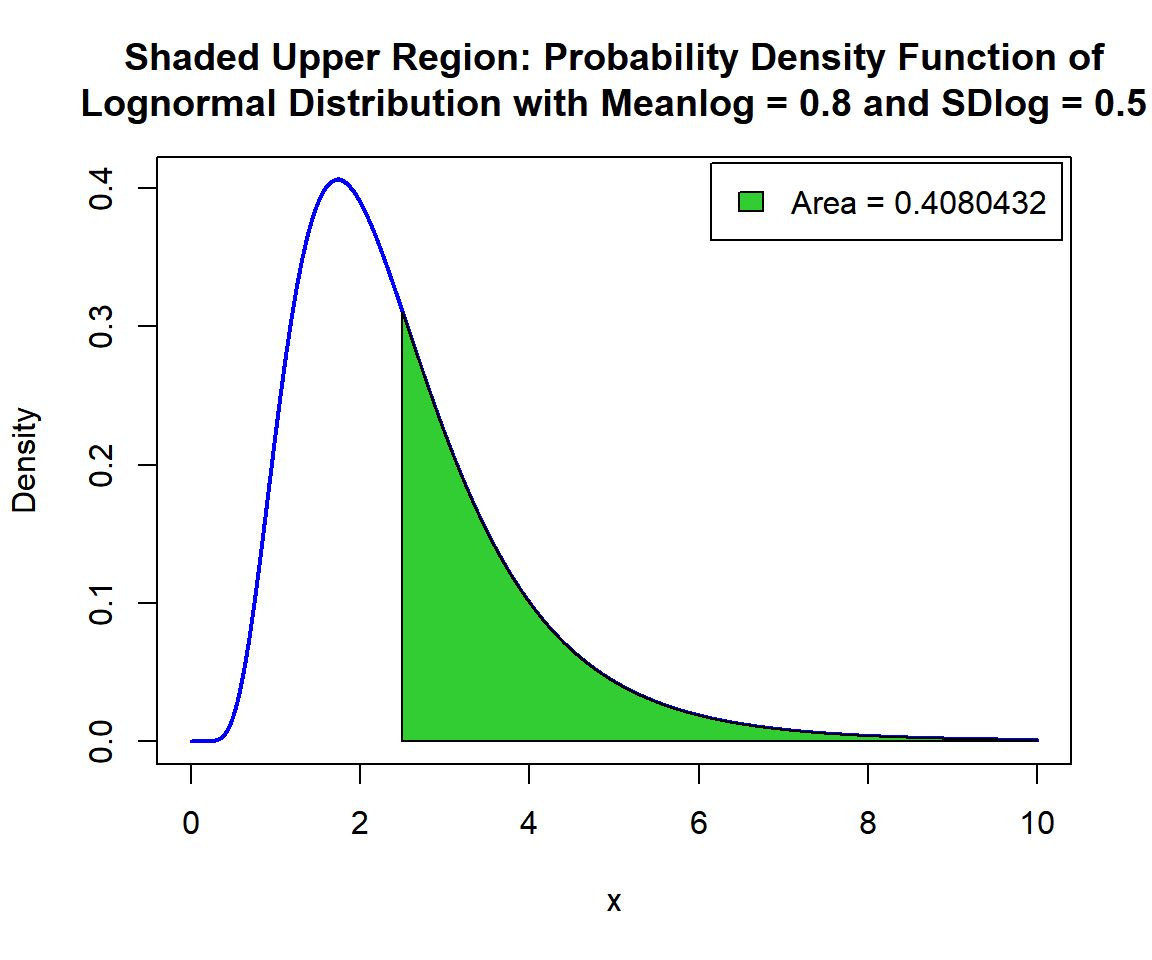

Shaded Upper Region: Probability Density Function (PDF) of Lognormal Distribution (0.8, 0.5) in R

7 qlnorm(): Derive Quantile for Lognormal Distributions in R

Derive the quantile for \(p = 0.9\), in the lognormal distribution with \(\tt{meanlog} = 1.5\) and \(\tt{sdlog} = 0.7\). That is, \(x\) such that, \(P(X \le x)=0.9\):

qlnorm(0.9, 1.5, 0.7)

[1] 10.9911

x = seq(0, 30, 1/1000); y = plnorm(x, 1.5, 0.7)
plot(x, y, type = "l",
     xlim = c(0, 30), ylim = c(0,1),
     main = "Cumulative Distribution Function of Lognormal Distribution
with Meanlog = 1.5 and SDlog = 0.7",
     xlab = "x", ylab = "Cumulative Distribution",
     lwd = 2, col = "blue")
# Add lines
segments(10.9911, -1, 10.9911, 0.9)
segments(-1, 0.9, 10.9911, 0.9)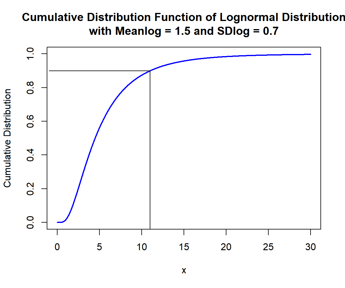

Cumulative Distribution Function (CDF) of Lognormal Distribution (1.5, 0.7) in R

x = seq(0, 30, 1/1000); y = dlnorm(x, 1.5, 0.7)
plot(x, y, type = "l",
     xlim = c(0, 30), ylim = c(0, max(y)),
     main = "Probability Density Function of Lognormal Distribution
with Meanlog = 1.5 and SDlog = 0.7",
     xlab = "x", ylab = "Density",
     lwd = 2, col = "blue")
# Add shaded region and legend
point = 10.9911
polygon(x = c(x[x <= point], point),
        y = c(y[x <= point], 0),
        col = "limegreen")
legend("topright", c("Area = 0.9"),
       fill = c("limegreen"),
       inset = 0.01)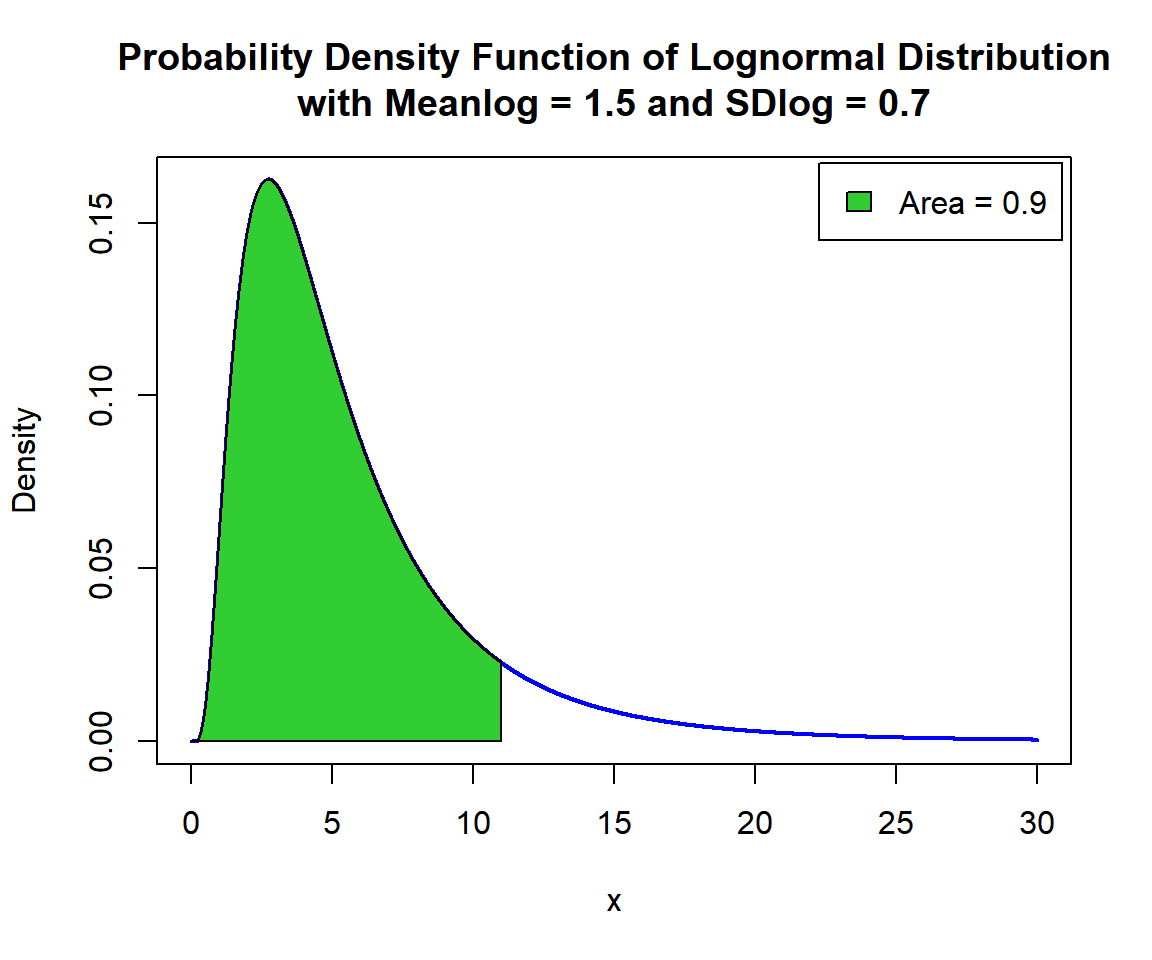

Shaded Probability Density Function (PDF) of Lognormal Distribution (1.5, 0.7) in R

For upper tail, for \(p = 0.1\), that is, \(x\) such that, \(P(X \ge x)=0.1\):

qlnorm(0.1, 1.5, 0.7, lower.tail = FALSE)

[1] 10.9911

x = seq(0, 30, 1/1000); y = dlnorm(x, 1.5, 0.7)
plot(x, y, type = "l",
     xlim = c(0, 30), ylim = c(0, max(y)),
     main = "Shaded Upper Region: Probability Density Function of
Lognormal Distribution with Meanlog = 1.5 and SDlog = 0.7",
     xlab = "x", ylab = "Density",
     lwd = 2, col = "blue")
# Add shaded region and legend
point = 10.9911
polygon(x = c(point, x[x >= point]),
        y = c(0, y[x >= point]),
        col = "limegreen")
legend("topright", c("Area = 0.1"),
       fill = c("limegreen"),
       inset = 0.01)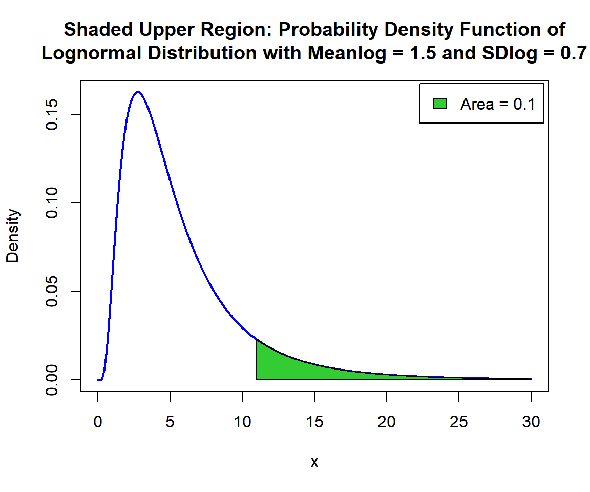

Shaded Upper Region: Probability Density Function (PDF) of Lognormal Distribution (1.5, 0.7) in R